
The Motor That Counted Its Own Steps
A Staircase Under the Microscope
In 1985 Ron Vale, Thomas Reese and Michael Sheetz took the axoplasm out of a squid’s giant nerve fibre and found in it a protein that carried beads along microtubules, the protein rails that run the length of every nerve cell. They proposed a name for it: kinesin. It is a motor, two heads joined at a neck, a long stalk, and a tail that holds cargo. Right now, in the nerve cells that run from your spine to your toes, a metre long, kinesins are walking cargo out to the far end.
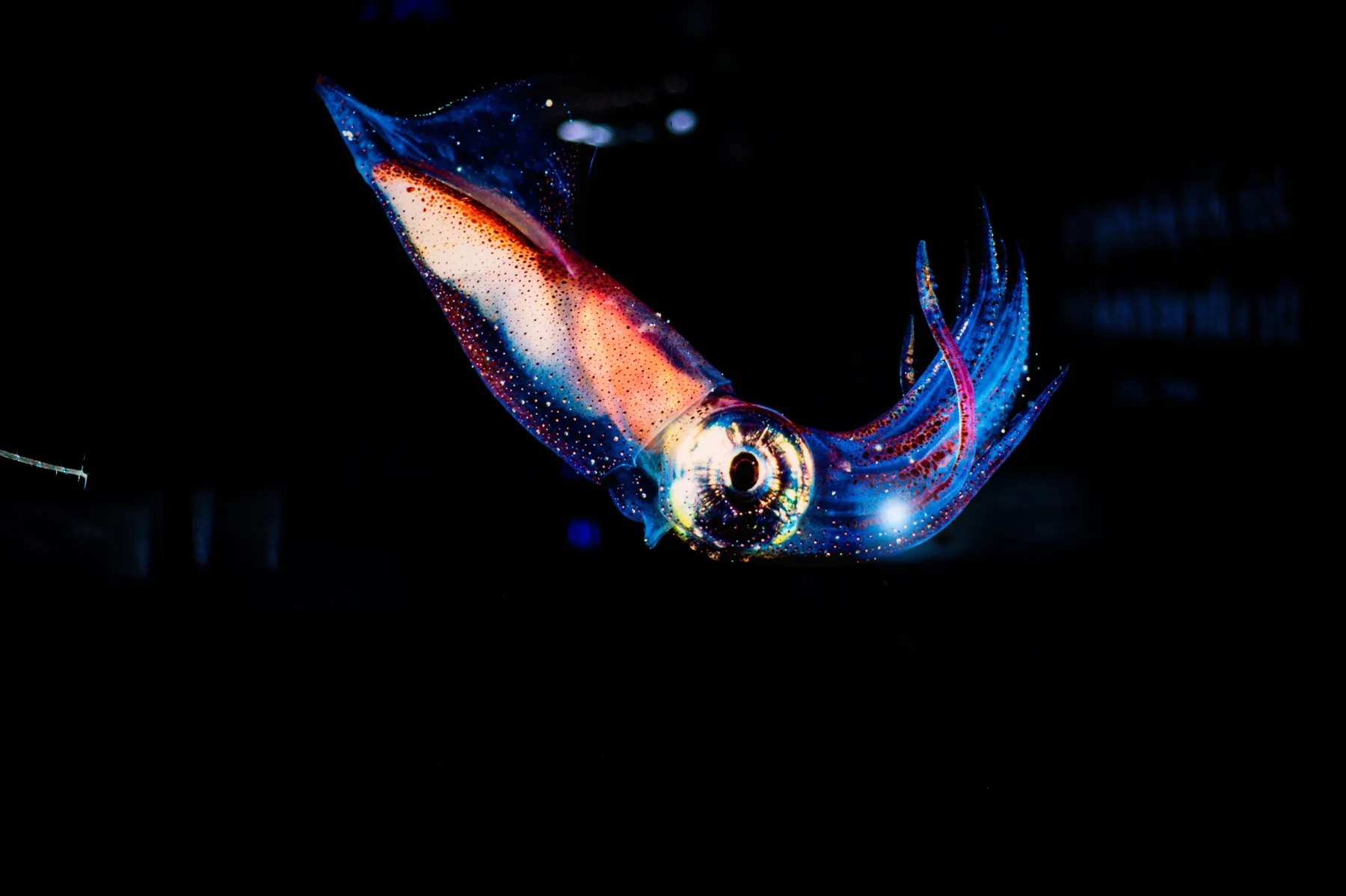
In 1993 Karel Svoboda, Christoph Schmidt, Bruce Schnapp and Steven Block caught a single kinesin in the act. They attached one molecule to a silica bead, held the bead in optical tweezers, set it down on a microtubule and followed it with an interferometer. The record was a staircase. “We find that kinesin moves with 8-nm steps”, one tubulin unit of the rail at a time.
Between two steps, though, the bead sits still, and everything that matters happens out of sight. The front head has to catch a molecule of ATP, the cell’s fuel; the fuel has to be split; the rear head has to let go of the rail and swing forward. A staircase shows none of it. How many hidden stages go into one step?
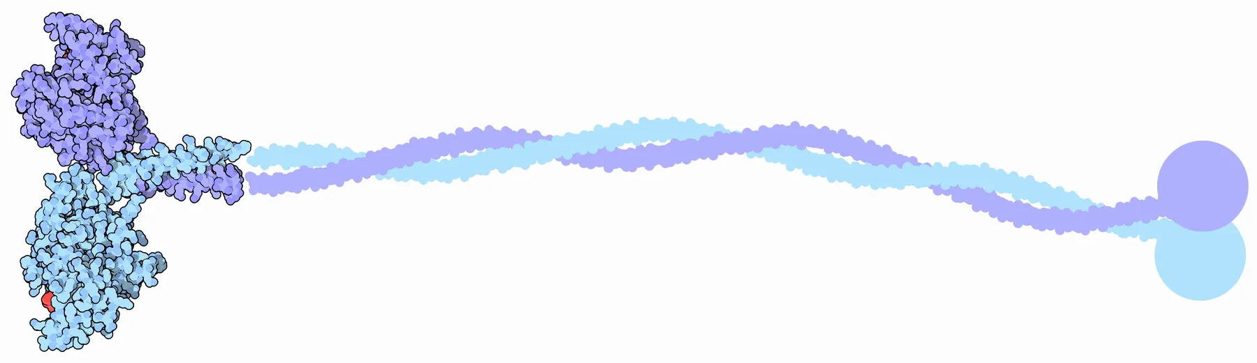
The answer came a year later, from the part of the record that is usually averaged away. Svoboda, Partha Mitra and Block looked not at the steps but at how irregular they were:
The variance in position was significantly smaller than expected for the case of stepwise movement along a regular lattice of positions with exponentially distributed intervals. The small variance suggests that two or more sequential processes with comparable reaction rates dominate the biochemical cycle.
The noise of the motor had counted its hidden steps. Behind that sentence is a theorem two probabilists had published seven years earlier, about a question that has nothing to do with biology: how regular can a clock be if it is built from $n$ memoryless parts? This post is that theorem, every equation it rests on, and a board where a motor walks on it.
A Cycle You Cannot See
Model the hidden chemistry as a Markov chain. The motor is in one of $n$ hidden states; it leaves each one after an exponential time, either for another hidden state or, from some states, by taking a step. The time $\tau$ between two steps is then the time the chain takes to get out, to be absorbed, and its distribution is called phase-type, written $\mathrm{PH}(\alpha, T)$. Marcel Neuts built the algorithmic theory of these distributions around 1980, and three objects define one:
- $T$, the $n \times n$ sub-generator: $T_{ij} \ge 0$ is the rate from hidden state $i$ to hidden state $j$, and $-T_{ii}$ is the total rate of leaving $i$, a step included;
- $\mathbf{t}_0 = -T\mathbf{1}$, the exit vector: the rate of stepping from each state;
- $\alpha$, a row vector: where the cycle starts.
For the motor I used one cycle, with illustrative rates rather than a fit to any experiment. State 0: the front head is empty, waiting for ATP, which binds at rate $k_A = k_{\text{on}}[\text{ATP}]$ with $k_{\text{on}} = 2$ per µM per second. States 1 and 2: two hidden stages of 5 ms each, standing in for everything that follows (splitting the ATP, the rear head letting go, the swing); leaving state 2 is the 8 nm step. State B: ADP, the spent fuel, can bind the empty head first, at rate $k_D = k_{\text{ADP}}[\text{ADP}]$ with $k_{\text{ADP}} = 0.5$ per µM per second; the head is then stuck until the ADP leaves, at $k_{\text{off}} = 25$ per second, and the motor is back in state 0. In the order 0, 1, 2, B:
Without ADP, $k_D = 0$, state B is never visited, and the cycle is a line of three stages. With ADP it has a loop: 0 to B and back, as many times as ADP wins the race.
The distribution of $\tau$ is a matrix exponential. The chance that no step has happened by time $t$, and the density of $\tau$, are
and its Laplace transform is the resolvent of the hidden chain, the matrix version of the resolvent in the lease post:
Expanding $\mathscr{R}_s$ in powers of $s$ gives every moment: $\mathbb{E}\,\tau^k = k!\;\alpha\, \mathscr{R}_0^{\,k}\, \mathbf{1}$.
For this cycle the transform can also be read off the diagram. Each hidden stage contributes a factor $k_i/(s + k_i)$. State 0 is left after an exponential time of rate $k_A + k_D$; with probability $k_D/(k_A + k_D)$ the motor detours through B, which costs a factor $k_{\text{off}}/(s + k_{\text{off}})$, and starts again. Summing the geometric series of detours:
I checked this against $\alpha\mathscr{R}_s\mathbf{t}_0$, computed as a linear solve, at four values of $s$ in three different cycles: they agree to $\textstyle 2.2 \times 10^{-16}$.
Every Number Is One Linear Solve
Nothing below needs $e^{Tt}$ or a matrix inverse. Each number is one linear solve with $-T$, which is applying $\mathscr{R}_0 = (-T)^{-1}$.
The mean, by first-step analysis. Let $m_i$ be the mean time to the next step from state $i$, and $q_i = -T_{ii}$. In state $i$ the motor waits $\textstyle 1/q_i$ on average, then jumps to $j$ with probability $T_{ij}/q_i$ or steps. So
This is the backward equation of the chain. For our cycle it reads, state by state,
$$m_2 = \frac{1}{k_2}, \qquad m_1 = \frac{1}{k_1} + m_2, \qquad m_B = \frac{1}{k_{\text{off}}} + m_0, \qquad m_0 = \frac{1 + k_A\, m_1 + k_D\, m_B}{k_A + k_D}$$
Substituting $m_B$ into the last and solving for $m_0$:
One step every $\mathbb{E}\tau$ seconds on average gives the speed $v = d/\mathbb{E}\tau$, with $d = 8$ nm. Put back the concentrations, write $H = 1/k_1 + 1/k_2 = 10$ ms for the hidden stages, and the speed takes a familiar form:
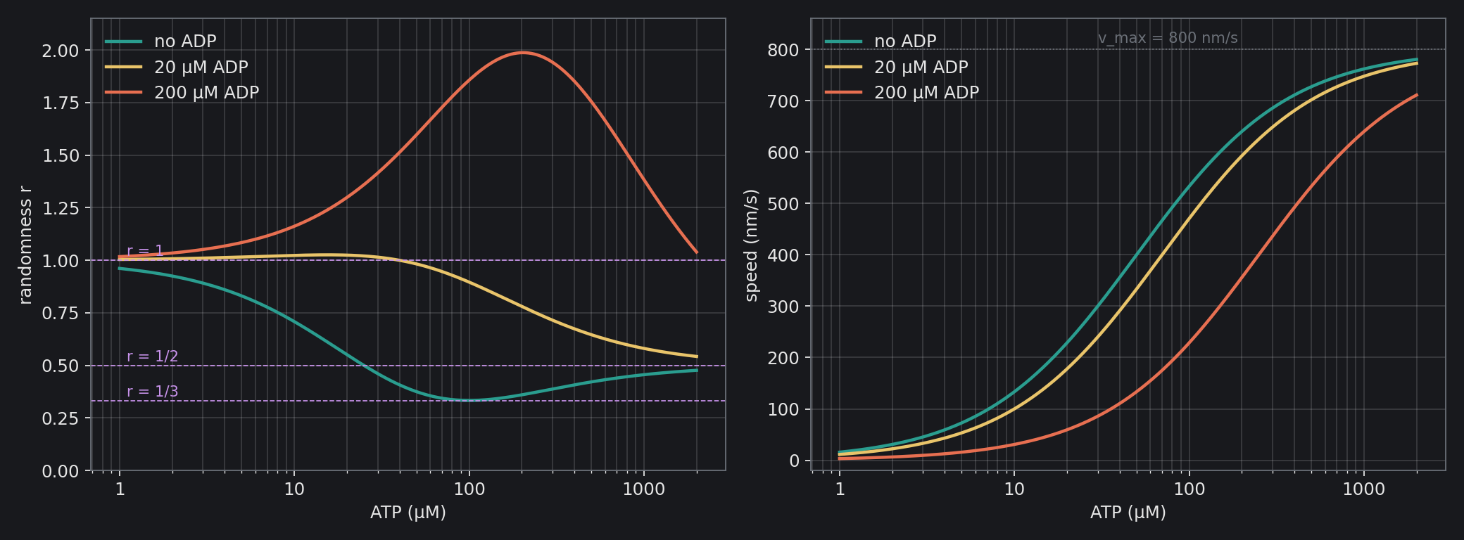
That is the Michaelis–Menten law with a competitive inhibitor. Nobody put enzyme kinetics into the model; it came out of one linear solve. ADP raises the ATP needed for half speed and leaves the top speed alone: with enough ATP, the fuel always wins the race. Across nine cycles the formula and the solve agree to $\textstyle 2.2 \times 10^{-16}$.
The second moment. Apply the same first step to $\tau^2$. Write $\tau = X + \tau^{\prime}$, with $X$ the exponential wait in the current state and $\tau^{\prime}$ the rest, independent of it. Since $\mathbb{E}X^2 = 2/q_i^2$, $\mathbb{E}_i\tau^2 = 2/q_i^2 + (2/q_i)\sum_j (T_{ij}/q_i)\, m_j + \sum_j (T_{ij}/q_i)\,\mathbb{E}_j\tau^2$, and by EQ 5 the first two terms add up to $\textstyle 2m_i/q_i$. Multiplying by $q_i$ and halving:
The number $r$, the squared coefficient of variation, is what biophysicists call the randomness of the motor. For one exponential stage, $r = 1$.
Where the time goes. The row vector $y = \alpha\mathscr{R}_0$, the solution of one transposed solve, holds the expected time spent in each state per cycle. Its entries add up to $\mathbb{E}\tau$, and $y_B/\mathbb{E}\tau$ is the share of the time the motor is stuck with ADP:
The whole density. The row vector $p(t) = \alpha e^{Tt}$ solves the forward equation $p^{\prime}(t) = p(t)\,T$ with $p(0) = \alpha$, and $f(t) = p(t)\,\mathbf{t}_0$. The board computes it by uniformisation: choose $L$ at least as large as every $-T_{ii}$, so that $P = I + T/L$ has no negative entries, and
Every term is positive, so nothing cancels, unlike a Taylor series of $e^{Tt}$. The one trap: for a long time $e^{-Lt}$ underflows to zero in double precision, so the board walks forward in pieces with $Lt \le 40$. Against scipy’s matrix exponential the worst error is $\textstyle 7.9 \times 10^{-14}$, measured in units of the mean time between steps.
From one cycle to a walk. The steps are a renewal process: the times between them are independent copies of $\tau$. If $N(t)$ steps have been taken by time $t$, the central limit theorem for renewal processes says that $N(t)$ is close to normal, with mean $t/\mu$ and variance $\sigma^2 t/\mu^3$, where $\mu = \mathbb{E}\tau$ and $\sigma^2 = \operatorname{Var}\tau$. The position is $x(t) = d\,N(t)$, so
The randomness is a slope. Follow many motors, plot the variance of their positions against time, divide the slope of the line by $d\,v$, and out comes $r$. A motor with one exponential stage per step has $\operatorname{Var} x = d\,v\,t$. The motors of 1994 had less.
Algorithm — The Motor’s Clock, Exactly
input:  T, the cycle's sub-generator (n × n); α, the start;
        d, the step; t, a time
t₀ ← −T·𝟏                     rate of stepping, per state
m  ← solve (−T)·m = 𝟏          ℛ₀𝟏: mean time to a step
m₂ ← solve (−T)·m₂ = m         ℛ₀²𝟏
Eτ ← α·m;  Eτ² ← 2·α·m₂
r  ← Eτ²/(Eτ)² − 1             randomness
v  ← d/Eτ                      speed
y  ← solve (−T)ᵀ·y = αᵀ        time spent in each state
Var x(t) ← r·d·v·t             renewal theorem
L  ← max over i of −T[i,i];  P ← I + T/L
p  ← α;  for pieces Δ of t with L·Δ ≤ 40:
    p ← Σₖ e^(−LΔ) (LΔ)ᵏ/k! · p·Pᵏ    uniformisation
f(t) ← p·t₀                    density of τ at t
n_min ← ⌈1/r⌉                  Aldous–Shepp floor
return v, r, y, f(t), n_min
The Theorem
Theorem (Aldous and Shepp, 1987). Let $\tau$ be the time a continuous-time Markov chain with $n$ transient states takes to be absorbed, from any starting distribution, with any rates and any routes between the states, loops included. Then
with equality only when $\tau$ has the Erlang distribution: $n$ stages of equal mean, one after another.
Read backwards, it is a counting rule. A cycle whose randomness is $r$ has at least
hidden states. In single-molecule biophysics the number $\textstyle 1/r$ is called $n_{\min}$. It is a floor and never a count, as the motor will show.
A line of stages: the easy half. If the chain visits $n$ stages once each, in order, with means $\mu_1, \dots, \mu_n$, then $\tau$ is a sum of independent exponentials. Their means add and so do their variances, and an exponential’s variance is its mean squared: $\mathbb{E}\tau = \sum_i \mu_i$ and $\operatorname{Var}\tau = \sum_i \mu_i^2$. By the Cauchy–Schwarz inequality, $\left(\sum_i \mu_i \cdot 1\right)^2 \le \left(\sum_i \mu_i^2\right)\left(\sum_i 1^2\right) = n \sum_i \mu_i^2$, so
With plenty of ATP, at 1,000 µM, our motor’s stages last 0.5, 5 and 5 ms, and $r = (0.25 + 25 + 25)/10.5^2 = 0.456$. That is below $\tfrac{1}{2}$, which no two-state cycle can reach, so the theorem proves at least three states and is right. It caught the half-millisecond stage, but only just.
Random routes. Suppose the route through the states is random but never visits a state twice. Condition on the route $J$. Given $J$, $\tau$ is a line of at most $n$ stages, so the easy half gives $\operatorname{Var}(\tau \mid J) \ge \mathbb{E}[\tau \mid J]^2/n$. The law of total variance splits the rest:
using $\mathbb{E}\big[\mathbb{E}[\tau \mid J]^2\big] = (\mathbb{E}\tau)^2 + \operatorname{Var}(\mathbb{E}[\tau \mid J])$. Not knowing the route only adds variance.
Loops: the hard half. A loop lets a route revisit states, so a route can pass through more than $n$ stages, and the bound for that route weakens to one over its number of visits. What saves the theorem is that a Markov chain cannot count. It remembers only the state it is in, so each time it is back in a state, the choice to go round again is made afresh, and the number of visits to any state is geometric. Every extra lap comes with the variance of a coin that might have stopped it. Proving that this variance always pays for the extra stages, in every possible cycle, is the hard half of the theorem. David Aldous and Larry Shepp did it in seven pages. In 1991 Colm O’Cinneide proved that the Erlang is also least variable in the sense of majorization.
The theorem, checked. I did not take it on trust. I drew 20,000 random cycles of each size from 2 to 6 states, with rates on every possible transition, loops included, random exits and random starting states: none came below $\tfrac{1}{n}$. Then I asked an optimiser to make $r$ as small as it could, from 40 random cycles of each size from 2 to 5. It stopped at $\tfrac{1}{2}$, $\tfrac{1}{3}$, $\tfrac{1}{4}$ and $\tfrac{1}{5}$, to within one part in 100,000, and the distribution it built was the Erlang: its distribution function agreed with the Erlang’s to within $\textstyle 1.4 \times 10^{-6}$. Most cycles are nowhere near the bound. The steadiest of the 20,000 random six-state cycles had $r = 0.390$, more than twice $\tfrac{1}{6}$. A cycle has to be built with care to keep time as well as the theorem allows.
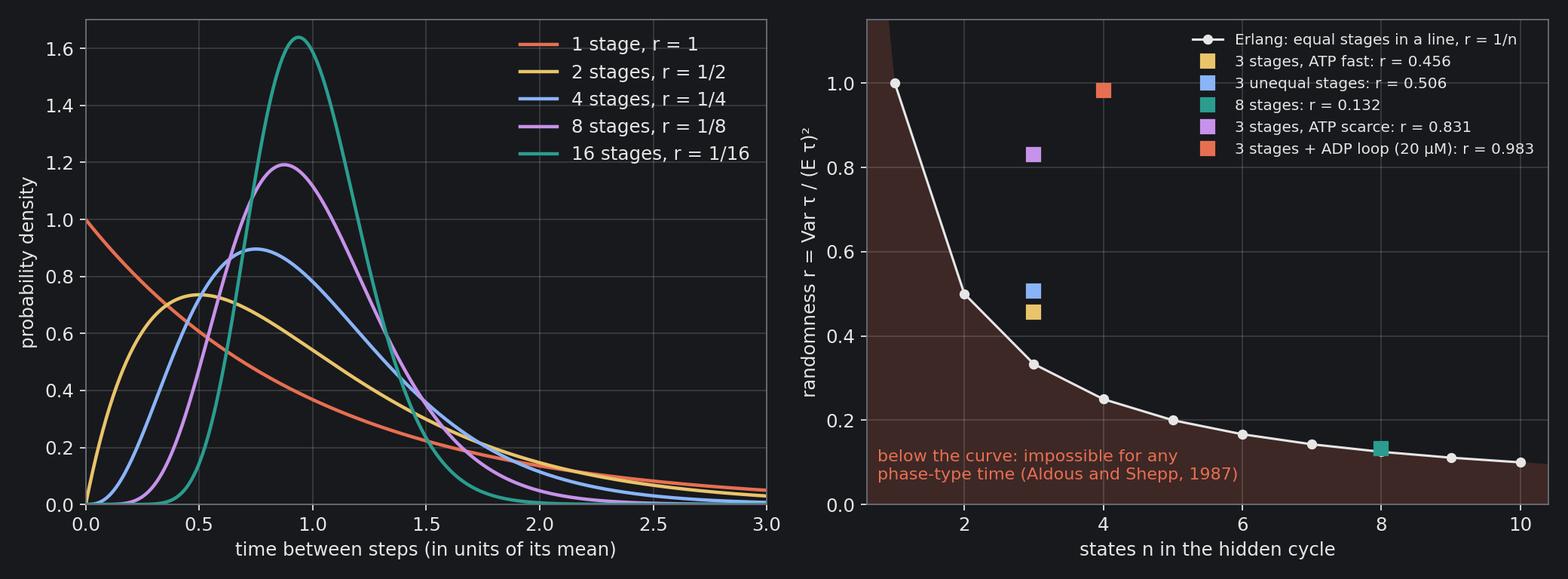
The theorem also explains a choice made in the lease post. There, a lease ending on a fixed date $T$ was replaced by one ending after $N$ random stages of mean $T/N$ each, so that its value became $N$ resolvent solves. Among all clocks built from $N$ memoryless stages, equal stages in a line keep the best time. Their spread, $T/\sqrt{N}$, is the smallest any $N$-stage clock can have.
Reading the Clock from the Noise
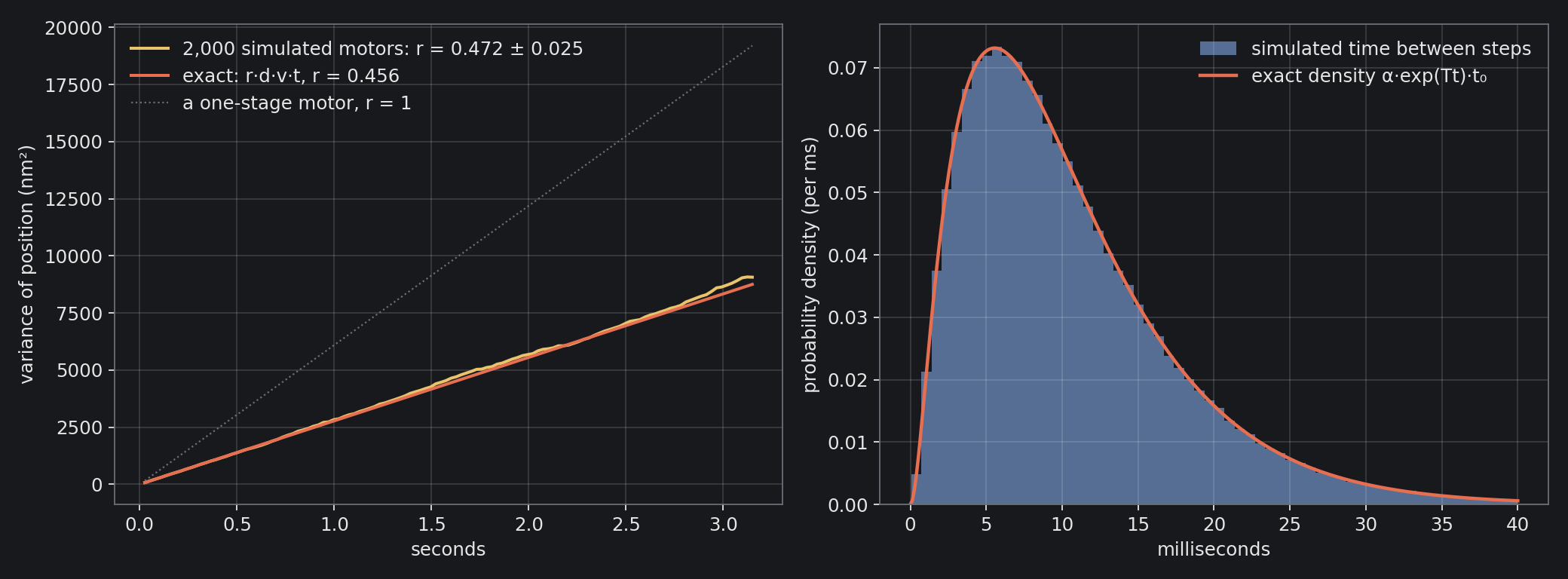
Now pretend not to know the cycle and do what the 1994 experiment did. I simulated 2,000 motors at 1,000 µM ATP, drawing each cycle as a sum of random stage times, with no formula used, and followed them for 3.15 s, about 300 steps each. They averaged 761.0 nm/s, against 761.9 from EQ 6. After 3.15 s the median motor had gone 2.40 µm, and 95% of them between 2.22 and 2.58 µm. A one-stage motor at the same speed would spread its motors 1.5 times as wide: a standard deviation of 139 nm instead of 93.5.
The variance of the 2,000 positions grows in a straight line. Its slope over the second half of the run, divided by $d\,v$, gives $r = 0.472 \pm 0.025$, the standard error coming from ten batches of 200 motors. The exact value is 0.456, 0.6 standard errors away.
How many stages does the noise prove? From the estimate alone, $\textstyle 1/0.472 = 2.12$, so three. An honest bound uses the top of the error bar instead: $r$ could be as large as $\textstyle 0.472 + 2 \times 0.025 = 0.522$, above $\tfrac{1}{2}$, so at about 95% confidence the data prove only two stages. The exact $r$ proves three, and the cycle has three. The noise of the measurement cost one stage.
The count depends on how the time is shared between the stages, and the same three states can read very differently:
| The cycle | States | r | At least |
|---|---|---|---|
| 0.5, 5 and 5 ms (1,000 µM ATP) | 3 | 0.456 | 3 |
| 5, 5 and 5 ms (100 µM ATP) | 3 | 0.333 | 3 |
| 0.5, 6.67 and 3.33 ms (unequal hidden stages) | 3 | 0.506 | 2 |
| 100, 5 and 5 ms (5 µM ATP) | 3 | 0.831 | 2 |
| 0.5 ms, then seven stages of 1.43 ms (1,000 µM ATP) | 8 | 0.132 | 8 |
At 100 µM ATP, ATP binds at 200 per second, exactly the rate of each hidden stage. The cycle is then the Erlang with three stages, $r = \tfrac{1}{3}$, and the theorem’s equality case turns up inside a motor. With unequal hidden stages the short one hides behind the long one; with scarce ATP, a 100 ms wait for fuel drowns out the 10 ms that follow. The noise counts only the stages that take comparable time, which is exactly how the 1994 abstract put it: “two or more sequential processes with comparable reaction rates.”
The Fuel and the Brake
ATP is the fuel; ADP is what is left once the fuel is spent. ADP can occupy the empty head’s pocket, and while it sits there ATP cannot bind: it has to leave first. In the cycle, that is the side state B and the loop through it. At 50 µM ATP, where the motor runs at half its top speed without ADP:
| ADP | nm/s | r | At least | Time stuck | Waits per step |
|---|---|---|---|---|---|
| none | 400 | 0.375 | 3 | 0% | 1 |
| 20 µM | 333 | 0.983 | 2 | 16.7% | 1.1 |
| 200 µM | 133 | 1.597 | 1 | 66.7% | 2 |
The speeds are EQ 7; “at least” is the theorem’s count, EQ 13; the time stuck is EQ 9; the waits per step are the mean number of visits to state 0, which is $\textstyle 1 + k_D/k_A$.
Here the brake does something unexpected. At 200 µM ADP, $r = 1.6$: the motor is more erratic than a motor with a single random stage, which could never exceed 1. Any wait for ATP can be interrupted by ADP, any number of times, each interruption costing 40 ms on average, so some steps come at once and others wait through several stalls. And the count collapses: $\textstyle 1/1.597 = 0.63$, so the theorem now proves at least one state. That is true and useless. The cycle still has its three stages, plus the ADP state for a fourth; no stage was removed, but the noise of the loop drowned them out. With 200 µM ADP the randomness peaks at 1.99, near 203 µM ATP.
The simulation agrees here too: 2,000 motors at 50 µM ATP and 200 µM ADP, followed for 18 s, average 133.6 nm/s against 133.3, and their noise gives $r = 1.679 \pm 0.063$ against the exact 1.597, 1.3 standard errors away.
The Walk
The board below runs the whole post. Under the sliders, the motor walks its microtubule hand over hand, the trailing head swinging past the bound one, while the cycle beside it shows where the chain is and when ADP has the head stuck. Below it are four cards: the speed and $r$ from the resolvent; $r$ measured from the noise of the simulated motors; and the number of stages Aldous and Shepp guarantee. Then a strip records the $r$ from each run of the motors, followed by the walk itself, the distance covered by the motors and the spread around the average, the straight line of the variance and the histogram of the times between steps against the exact density.
Move ATP down to about 100 µM and $r$ falls to $\tfrac{1}{3}$: the motor becomes the Erlang. Switch to unequal hidden stages and the count falls short by one. Lower ATP to about 50 µM, add about 200 µM of ADP, and watch $r$ climb past 1 while the count drops to one. The page builds the cycle’s matrix and computes everything itself, solving the linear systems of EQ 5, 8 and 9 and running the uniformisation of EQ 10, and simulates up to 2,000 motors per run. I checked it against Python in a browser. Its moments agree with numpy’s to $\textstyle 1.8 \times 10^{-15}$, its density with scipy’s matrix exponential to $\textstyle 4.4 \times 10^{-14}$, and its inhibition formula to $\textstyle 4.4 \times 10^{-16}$. In 30 settings its measured $r$ was within 1.93 standard errors of the exact one, and its count never exceeded the number of states in the cycle.
The Noise Was the Signal
The same statistics kept answering questions about the motor. In 1997 Mark Schnitzer and Steven Block used the intervals between steps at low ATP, and the fluctuations in speed as ATP varied, to settle how much fuel a step costs:
At near-zero load, kinesin molecules hydrolyse a single ATP molecule per 8-nm advance.
In 2004 Ahmet Yildiz, Michio Tomishige, Ron Vale and Paul Selvin put a fluorescent dye on one head and watched it move: steps of 17.3 ± 3.3 nm, about twice the molecule’s 8.3, alternating with steps of 0 nm. Each head leapfrogs the other while the molecule as a whole advances 8 nm at a time. Kinesin walks hand over hand.
Larry Shepp appeared here two days ago, in the cod post, solving the fishing problem with Luis Alvarez. In 1987 he and David Aldous answered a question about clocks: how well can $n$ memoryless parts keep time? Their answer, seven pages in a journal of stochastic models, is what lets a bead jittering in an optical trap testify about chemistry no microscope can see. Everyone else averaged the noise away; for the motor, the noise was the signal.
Sources
- D. Aldous and L. Shepp, “The least variable phase type distribution is Erlang”, Communications in Statistics. Stochastic Models 3 (1987) 467–473.
- C. A. O’Cinneide, “Phase-type distributions and majorization”, The Annals of Applied Probability 1 (1991), no. 2.
- M. F. Neuts, Matrix-Geometric Solutions in Stochastic Models: An Algorithmic Approach, Johns Hopkins University Press, Baltimore, 1981.
- R. D. Vale, T. S. Reese and M. P. Sheetz, “Identification of a novel force-generating protein, kinesin, involved in microtubule-based motility”, Cell 42 (1985) 39–50.
- K. Svoboda, C. F. Schmidt, B. J. Schnapp and S. M. Block, “Direct observation of kinesin stepping by optical trapping interferometry”, Nature 365 (1993) 721–727.
- K. Svoboda, P. P. Mitra and S. M. Block, “Fluctuation analysis of motor protein movement and single enzyme kinetics”, Proceedings of the National Academy of Sciences 91 (1994) 11782–11786.
- M. J. Schnitzer and S. M. Block, “Statistical kinetics of processive enzymes”, Cold Spring Harbor Symposia on Quantitative Biology 60 (1995) 793–802.
- M. J. Schnitzer and S. M. Block, “Kinesin hydrolyses one ATP per 8-nm step”, Nature 388 (1997) 386–390.
- A. Yildiz, M. Tomishige, R. D. Vale and P. R. Selvin, “Kinesin walks hand-over-hand”, Science 303 (2004) 676–678.
- J. R. Moffitt, Y. R. Chemla and C. Bustamante, “Methods in statistical kinetics”, Methods in Enzymology 475 (2010) 221–257.
- D. S. Goodsell, “Kinesin”, RCSB PDB Molecule of the Month, April 2005, doi:10.2210/rcsb_pdb/mom_2005_4.
Every number in the text, the three charts and the board are computed by the scripts archived with this post, from illustrative rates that are not fitted to any experiment. Each formula is checked against a direct linear solve, the density against scipy’s matrix exponential, the theorem against random cycles and an optimiser, and the noise against 2,000 simulated motors per case, saved once. The board was checked against the same Python code in a browser.
Interested in applying these ideas to your work? Get in touch.