The Catch That Emptied the Grand Banks

Five Hundred Years, Then Nothing

On 1 July 1992, Canada Day, the federal fisheries minister John Crosbie went to Bay Bulls, a fishing village near St. John’s, and was met by a crowd of angry fishermen who had heard the rumours. “I didn’t take the fish from the God damn water,” he shouted at them. The next day, in a hotel ballroom in St. John’s, with fishermen trying to force the doors, he announced a two-year moratorium on the northern cod fishery.

**Figure 1.** An Atlantic cod, Gadus morhua, at the Ozeaneum aquarium in Stralsund. Photograph by Wilhelm Thomas Fiege, CC BY-SA 4.0, via Wikimedia Commons.

The cod off Newfoundland had shaped the island’s life for five hundred years. The catch had peaked in 1968 at 810,000 tons, after factory trawlers arrived. By 1992 the northern cod stock had fallen to about 1% of its historic size; its spawning biomass was down 99%. Some 30,000 to 37,000 fishermen and plant workers lost their work, by different counts, in the largest industrial closure in Canadian history. In 1993 the moratorium was extended indefinitely. The two years lasted thirty-two.

The collapse had many causes: surveys that overestimated the stock, catches that rose with new technology and were mistaken for a growing stock, warnings that went unheeded. This post is about something underneath all of them, the arithmetic every quota sits on. It is simple enough to solve exactly, and it says that the most natural rule in fisheries, the same catch every year at the level the stock can sustain, is a trap.

"The bank hand-line cod fishery": an old-style Grand Bank cod schooner, its crew fishing with hand lines at the rail. Drawing by H. W. Elliott and Capt. J. W. Collins for G. B. Goode, The Fisheries and Fishery Industries of the United States (1887). Public domain, via Wikimedia Commons. — **Figure 2.** “The bank hand-line cod fishery”: an old-style Grand Bank cod schooner, its crew fishing with hand lines at the rail. Drawing by H. W. Elliott and Capt. J. W. Collins for G. B. Goode, The Fisheries and Fishery Industries of the United States (1887). Public domain, via Wikimedia Commons.

The Hump and the Cliff

Measure the stock as a share $x$ of its unfished size. Left alone, it grows logistically: fast when it is small and food is plentiful, slowly as it nears the size its habitat can hold.

$$\frac{dx}{dt} = r\,x(1 – x) – h$$

$(1)$

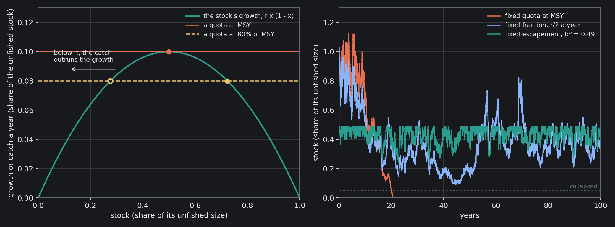
Here $r$ is the stock’s growth rate and $h$ is the catch a year. The growth $r\,x(1-x)$ is a hump, largest at half the unfished size, where it is $r/4$. That is the maximum sustainable yield, MSY: take $r/4$ a year from a stock held at one half and, without good years or bad, it stays there forever.

Look closely at that balance point, though. Above one half, a stock that rises grows more slowly than $r/4$ and falls back; a stock that dips grows faster and comes back up. Below one half, that is no longer so. A stock pushed below one half grows by less than the catch, so next year it is smaller still, and grows by even less. Nothing stops it until it is gone. The balance point at MSY is stable from above and a cliff from below.

A smaller quota moves the cliff away but does not remove it. At 80% of MSY there are two balance points, at $x = 0.724$ and $x = 0.276$. The upper one is stable. The lower one is the cliff’s new edge: any stock pushed below 0.276 slides to zero, however long it takes.

Left: the stock's growth against its size, and two fixed quotas. At MSY the quota touches the hump at its top, a balance that is stable only from above; at 80% of MSY it crosses the hump twice, and the lower crossing (open circle) is a cliff edge. Right: one simulated century of the same good and… — **Figure 3.** Left: the stock’s growth against its size, and two fixed quotas. At MSY the quota touches the hump at its top, a balance that is stable only from above; at 80% of MSY it crosses the hump twice, and the lower crossing (open circle) is a cliff edge. Right: one simulated century of the same good and bad years under three rules: a fixed quota at MSY collapses after about twenty years; a fixed fraction and a fixed escapement keep fishing.

Good Years and Bad

Real stocks are never still. Recruitment, the number of young fish that survive to be caught, swings with temperature, food and predators. The simplest honest model adds random good and bad years in proportion to the stock:

$$dX = r\,X(1 – X)\,dt + \sigma X\,dW – \text{(the catch)}$$

$(2)$

with $W$ a Brownian motion. I used illustrative numbers, not a fit to any real stock: a growth rate $r = 0.4$ a year, so that MSY is 0.1 of the unfished stock a year, year-to-year noise $\sigma = 0.25$, and a discount rate of 5% for valuing future catches.

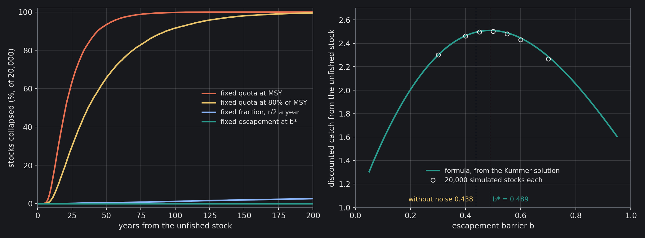
Now a fixed quota at MSY is doomed. The balance point sits exactly on the cliff’s edge, and the first run of bad years pushes the stock over it. Of 20,000 simulated stocks starting unfished and fished this way, 93.4% had collapsed (fallen below 5% of their unfished size) within 50 years and 99.7% within a century. The average time to collapse can be computed exactly from the diffusion’s scale and speed densities: 24.9 years. The simulations give 25.0.

Backing off does not save it, only slows it. At 80% of MSY, 65.7% of the stocks collapse within 50 years and 91.6% within a century; the mean time is 47.9 years. At 60% of MSY it is 168 years. With noise and a fixed catch, the bottom of the hump is always reachable, and once there the catch finishes the job. Every fixed quota, at any level, collapses the stock with probability one; the only question is when.

Fish What the Sea Can Spare

The way out is to let the catch follow the fish. A fixed fraction of the stock (constant effort) already does much better: the catch shrinks as the stock does, and fishing 20% of it a year, which holds the stock at one half without noise, lets only 1.1% of the simulated stocks fall below 5% within a century.

The best rule goes further. Choose a level $b$, the escapement, and each year catch everything above it and nothing below. In good years the catch is large; in bad years there is none at all. William Reed proved in 1979 that such a rule is optimal for a broad class of stochastic models, and in 1998 Luis Alvarez and Larry Shepp solved the continuous-time logistic case exactly. The problem is singular stochastic control: maximise the discounted catch $\mathbb{E}\int_0^\infty e^{-\delta t}\,dZ_t$, where $Z_t$ is the catch so far.

Below the barrier nothing is caught, so the value $V$ of the stock satisfies the resolvent equation of the process, $(\mathscr{L} – \delta)V = 0$, where $\mathscr{L}$ is its generator. Its solutions are built from the two fundamental solutions that also build the resolvent $\mathscr{R}_\delta$, and here the one that matters, the increasing one, is a Kummer function:

$$\varphi(x) = x^{\theta}\, M\!\left(\theta,\; 2\theta + \frac{2r}{\sigma^2},\; \frac{2r}{\sigma^2}\,x\right), \qquad \tfrac{1}{2}\sigma^2\theta(\theta – 1) + r\theta = \delta$$

$(3)$

Write $\varphi(x) = x^\theta g(x)$ in the resolvent equation and choose $\theta$ to cancel its constant term; what is left is Kummer’s equation for $g$ in the variable $\textstyle 2rx/\sigma^2$. With $\varphi$ in hand, a barrier $b$ is worth $V_b(x) = \varphi(x)/\varphi^{\prime}(b)$ below it, because each fish above the barrier is caught at once, $V_b^{\prime}(b) = 1$. The best barrier makes $\varphi^{\prime}(b)$ as small as possible:

$$\varphi^{\prime\prime}(b^*) = 0$$

$(4)$

For our illustrative stock, $b^* = 0.489$. Without noise the optimum would be $\tfrac{1}{2}(1 – \delta/r) = 0.438$: the good and bad years make the best policy more cautious, and it leaves more fish in the water. From the unfished stock the first catch takes it from 1 down to 0.489 at once, and after that the stock wanders below the barrier and is skimmed every time it rises above. Its discounted catch is $V_{b^*}(1) = 2.510$, almost twice the 1.30 of the fixed quota at MSY. Averaged over two centuries it lands 0.0999 of the unfished stock a year: the maximum sustainable yield that the fixed quota promised and could not keep. And not one of the 20,000 simulated stocks collapsed. Fishing cannot push the stock below $b^*$; only an extraordinary run of bad years could.

Algorithm — The Best Escapement, Exactly

input:  r, σ: growth and noise of the stock; δ: discount rate
θ ← the positive root of ½σ²θ(θ − 1) + rθ − δ = 0
k ← 2r/σ²
M(a, b, z) ← Σₙ (a)ₙ/(b)ₙ · zⁿ/n!       Kummer's function
φ(x) ← x^θ · M(θ, 2θ + k, k·x)
φ′, φ″ ← the same, differentiated
          (M′(a, b, z) = (a/b) · M(a + 1, b + 1, z))
b* ← the root of φ″(b) = 0 in (0, 1), by bisection
V(x) ← φ(x)/φ′(b*)                 for x < b*
V(x) ← x − b* + φ(b*)/φ′(b*)       for x ≥ b*
return b*, V

To check it, I solved the ODE for $\varphi$ directly from a small stock, numerically, and it agrees with the Kummer formula to $\textstyle 4 \times 10^{-12}$. I simulated 20,000 stocks fished at $b^*$ for 200 years: their discounted catch averages 2.511, against 2.510 from the formula (0.4 standard errors apart). Away from $b^*$ the simulations sit up to 0.6% below the formula, and that gap halves each time the simulation’s time step is quartered (1.48%, 0.60%, 0.28% at a barrier of 0.7): it is the error of the simulation, which catches the fish a step late, not of the formula.

Left: the share of 20,000 simulated stocks collapsed (below 5% of their unfished size) against time from the unfished stock, under each rule. Right: the discounted catch from the unfished stock for every escapement barrier, from the Kummer solution (line) and from simulation (circles), with the… — **Figure 4.** Left: the share of 20,000 simulated stocks collapsed (below 5% of their unfished size) against time from the unfished stock, under each rule. Right: the discounted catch from the unfished stock for every escapement barrier, from the Kummer solution (line) and from simulation (circles), with the best barrier b* = 0.489 and the barrier without noise, 0.438.

Three Ways to Fish

The board below fishes the same century of good and bad years three ways at once. Move the quota up to MSY or down to half of it; move the fraction and the barrier; turn the noise up and down; draw new years. Below the two charts, a table runs 1,000 centuries for each rule on the same years. The page computes Kummer’s function, the best barrier and every simulated year itself. I checked it against Python: its $\varphi$ and $\varphi^{\prime\prime}$ agree with scipy’s to $\textstyle 6 \times 10^{-16}$ and its $b^*$ to $\textstyle 10^{-13}$, and with its random years rebuilt in Python, its centuries and its table agree exactly.

The stochastic logistic stock fished three ways on the same random years: a fixed quota (as a share of MSY), a fixed fraction a year and a fixed escapement (the best barrier b* for the noise is computed on the page). The cards say whether each is still fishing; the charts show the stock and the catch over a century; the table runs 1,000 centuries for each rule.

The Rule Came Thirty Years Late

A moratorium is the bottom half of an escapement rule: when the stock is below the barrier, catch nothing. Canada applied it in 1992, to a stock already near the bottom of its hump, and for decades the cod did not return; the waters filled with crab and shrimp instead.

In 2024 the government lifted the moratorium on the northern cod and allowed commercial fishing for the first time since 1992, with a total allowable catch of 18,000 tons: about one forty-fifth of the catch of 1968.

An abandoned fishing boat in the village of Ferryland, on Newfoundland's southern shore. Photograph by Ritche Perez, Pexels. — **Figure 5.** An abandoned fishing boat in the village of Ferryland, on Newfoundland’s southern shore. Photograph by Ritche Perez, Pexels.

Sources

J. R. Beddington and R. M. May, “Harvesting natural populations in a randomly fluctuating environment”, Science 197 (1977) 463–465.
W. J. Reed, “Optimal escapement levels in stochastic and deterministic harvesting models”, Journal of Environmental Economics and Management 6 (1979) 350–363.
E. Lungu and B. Øksendal, “Optimal harvesting from a population in a stochastic crowded environment”, Mathematical Biosciences 145 (1997) 47–75.
L. H. R. Alvarez and L. A. Shepp, “Optimal harvesting of stochastically fluctuating populations”, Journal of Mathematical Biology 37 (1998) 155–177.
G. B. Goode, The Fisheries and Fishery Industries of the United States, Government Printing Office, Washington, 1887.
“The announcement of the moratorium”, Centre for Distance Learning and Innovation, Newfoundland and Labrador (cdli.ca).
“Collapse of the Atlantic northwest cod fishery” and “John Crosbie”, Wikipedia: the catch of 1968, the state of the stock in 1992, the jobs lost, the extension of 1993, the reopening of 2024 and the Bay Bulls remark.

Every number in the text, the two charts and the board are computed by the scripts archived with this post, from the illustrative parameters: the Kummer solution checked against a direct solution of its ODE, the mean time to collapse against simulation, and the value of every barrier against 20,000 simulated stocks, saved once; the board was checked against the same Python code in a browser.

Interested in applying these ideas to your work? Get in touch.