Should You Wait for a Dip?

Money on the Sidelines

Everyone who has ever had cash to invest has asked it. The market has run up, and surely it will give some of it back. Why not wait for a pullback, buy 10% cheaper, and own more for the same money?

Here is how that went in the S&P 500. Take every month from January 1990 to September 2021 as the month the money was ready: 381 starts. One investor buys at once. The other waits for the index to fall 10% below where it stood that month, buys at the dip, or buys anyway after a year if the dip never comes. Five years after the money was ready, the waiter was behind in 72% of the starts, and on average held 4.7% less.

The worst start was April 2020. The market had just crashed with the pandemic, and a cautious investor waited for another 10% fall that never came within the year. Five years on, that investor had a third less than the one who bought in April.

**Figure 1.** A candlestick chart sliding into a dip, with the first green bars at the bottom. Photograph: Alex Luna, Pexels.

That is the first half of the answer, and there is a short theorem behind it. The second half is about prices that do come back. There, waiting is exactly right, and how long to wait turned out to be the most surprising thing I computed for this post.

Every Day in Cash Has a Price

Model the market the simplest honest way: a price that grows at $\mu$ a year on average, with random swings (a geometric Brownian motion), and cash that earns $r$. A dollar waits in cash until some rule says buy, at a time $\tau$ the rule decides from what it has seen so far: “10% below where I started”, “after three red days”, anything that does not look into the future. At the horizon $T$ the dollar has become

$$W = e^{r\tau}\,\frac{S_T}{S_\tau},\qquad \mathbb{E}[W] = e^{\mu T}\;\mathbb{E}\!\left[e^{-(\mu – r)\,\tau}\right]$$

$(1)$

The reason is that a geometric Brownian motion forgets where it has been. Whatever happened before $\tau$, from $\tau$ on the price grows at $\mu$ on average, so the only thing a waiting rule changes is how long the money sits earning $r$ instead of $\mu$. If the market beats cash, $\mu > r$, the last factor is below one for every rule that ever waits, and buying at once is the best rule there is. No clever dip rule beats it on average, because the dips it waits for are paid for by the rallies it misses.

“On average” carries the weight. The theorem does not say the waiter loses every time.

Ahead Six Times in Ten, and Still Behind

To see the difference, I simulated 20,000 markets for 20 years, with the market growing at 7% a year, cash at 3% and annual swings of 16%, all assumed. The rule: wait for a 10% dip below the starting price, and buy anyway after five years.

The dip came within five years in 54.6% of the markets, typically after about seven months, and in those the waiter bought 10% cheaper and stayed ahead. In the rest the market ran away, and the waiter bought five years late at a much higher price. The waiter finished ahead on 60% of the paths. And yet a dollar became 3.65 for the waiter on average, against 4.07 for the investor who bought at once: about 10% less. The formula above, fed the simulated waiting times, predicts 3.64; the simulation gives 3.65 ± 0.04.

Left: 20,000 simulated markets (7% growth, 3% cash, 16% swings, 20 years, all assumed): the final wealth of an investor who waited for a 10% dip, buying anyway after five years, divided by that of one who bought at once. The waiter ends ahead on 60% of the paths, and with 3.65 per dollar against… — **Figure 2.** Left: 20,000 simulated markets (7% growth, 3% cash, 16% swings, 20 years, all assumed): the final wealth of an investor who waited for a 10% dip, buying anyway after five years, divided by that of one who bought at once. The waiter ends ahead on 60% of the paths, and with 3.65 per dollar against 4.07 on average. Right: the S&P 500 with dividends reinvested, for every month from January 1990 to September 2021: the same ratio five years on, for an investor who waited up to a year for a 10% dip. Teal: waiting won; coral: waiting lost.

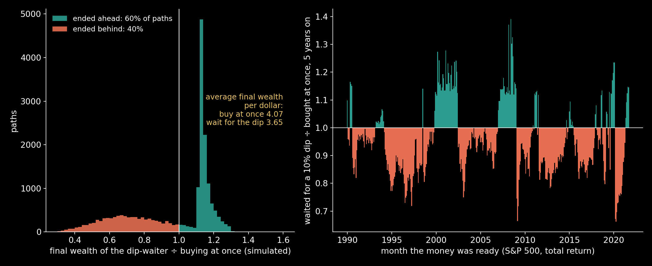
The picture on the left is the shape of a bad bet that feels like a good one. The wins are frequent and modest, the tall teal spike just above one: the dip came, and the waiter bought a little cheaper. The losses are spread far to the left, and they are large; the worst path ended with less than a fifth of what buying at once would have given.

Thirty-Six Years of the S&P 500

The simulation runs on assumed numbers. The replay is the real index. I used Robert Shiller’s monthly data for the S&P Composite, which gives the price, the dividend and the 10-year Treasury yield, and reinvested the dividends. While the waiter waits, the cash earns the 10-year yield. That is generous to the waiter, because cash usually earns less.

Waiting for a 5% dip left the waiter behind in 63% of the starts; for a 10% dip, in 72%; for a 20% dip, in 77%. The average shortfall barely moved: 4.2%, 4.7% and 4.7% of final wealth. The deeper the dip you insist on, the less often it comes within a year: 33%, 19% and 8% of the time.

The real market was harsher than the simulation, and the reason is the deadline. In the simulation the waiter gave the dip five years; here, one. The theorem says the deadline changes how often waiting wins, never whether it loses on average.

When waiting won, it won in a crash. The teal bars on the right of the picture cluster around 2000–2002, 2007–2008 and the months before the 2020 crash, and the best start, June 2008, ended 39% ahead. Those are the years people remember, which is why dip-buying feels as if it works. Measured over every start, the waiter was ahead by 13.1% on average when ahead, behind by 11.5% when behind, and behind more than two and a half times as often.

Even foresight does not buy much. An investor who knew the future and bought at the best month within the year would have ended with 8% more on average, and in a third of the months the best month was the first one.

Two cautions. The 381 starts overlap, so 36 years hold only about seven independent five-year windows: the replay illustrates the theorem, and the theorem carries the proof. And Shiller’s price is the monthly average of daily closes, so a dip that comes and goes inside a month is not seen.

Prices That Come Back

Not every price drifts. The gap between two share classes of one company, a future and the asset it is written on, two funds that hold almost the same things: prices like these are pulled back toward a level. The simplest model of that pull is the Ornstein–Uhlenbeck process, written down in 1930 for the velocity of a particle jostled by a fluid:

$$dX_t = \kappa\,(\theta – X_t)\,dt + \sigma\,dW_t$$

$(2)$

The price is pulled toward $\theta$ at a rate proportional to its distance from it. A deviation halves, on average, in $\ln 2/\kappa$, and the typical swing, the standard deviation of where the price spends its time, is $\sigma/\sqrt{2\kappa}$. For a price like this the dip is the whole point: buy below $\theta$, sell above it. The question is how far below.

My example is assumed, not fitted: a price that reverts to $1.00 with a typical swing of 10 cents and a half-life of 44 trading days, about two months ($\kappa = 4$ a year). It costs a cent to buy and a cent to sell, money is worth 5% a year, and one unit is held at a time.

**Figure 3.** Boats on the mud at low tide, waiting for the water to come back. Photograph: Richard REVEL, Pexels.

One Trade, Solved

Tim Leung and Xin Li posed this cleanly in 2015, with a stop-loss that this post leaves out, and developed it in their 2016 book. First the exit: holding one unit, when should you sell? Then the entry: when should you buy, knowing you will exit optimally?

$$\begin{gathered} V_1(x) = \sup_{\tau}\,\mathbb{E}_x\!\left[e^{-r\tau}\,(X_\tau – c)\right] \\[6pt] J_1(x) = \sup_{\nu}\,\mathbb{E}_x\!\left[e^{-r\nu}\big(V_1(X_\nu) – X_\nu – c\big)\right] \end{gathered}$$

$(3)$

Both answers are a level. Sell the first time the price reaches $b_1$; buy the first time it falls to $d_1$. Away from the levels the values solve $(\mathscr{L} – r)f = 0$, where $\mathscr{L} = \kappa(\theta – x)\,\partial_x + \tfrac12\sigma^2\partial_{xx}$ is the generator of the process, and that equation has an increasing and a decreasing solution, each an integral:

$$\begin{gathered} F(x) = \int_0^\infty u^{\,r/\kappa – 1}\, e^{\sqrt{2\kappa/\sigma^2}\,(x – \theta)\,u \,-\, u^2/2}\,du \\[6pt] G(x) = \int_0^\infty u^{\,r/\kappa – 1}\, e^{\sqrt{2\kappa/\sigma^2}\,(\theta – x)\,u \,-\, u^2/2}\,du \end{gathered}$$

$(4)$

Smooth fit pins the levels: $F(b_1) = (b_1 – c)\,F^{\prime}(b_1)$ for the exit, and a condition of the same kind, in $G$ and $V_1$, for the entry.

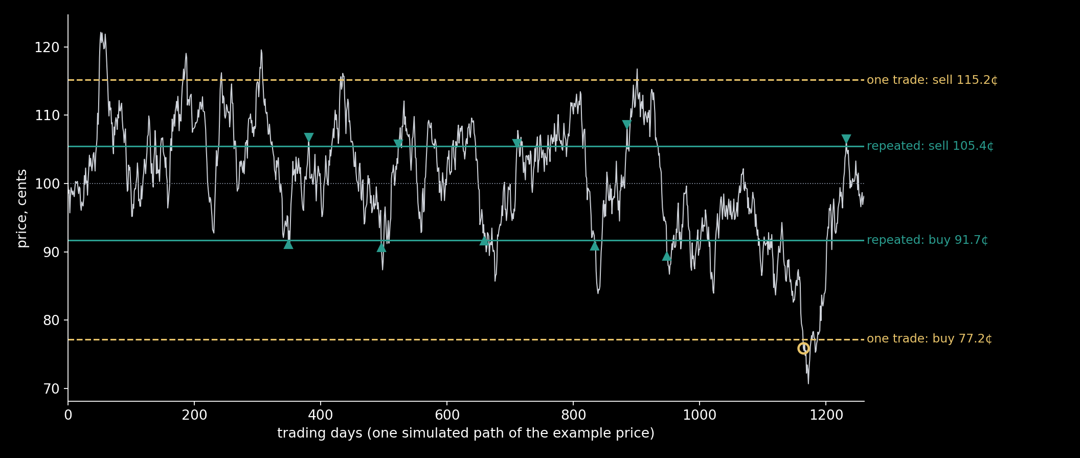
For the example: buy at 77.2 cents and sell at 115.2 cents, which is 2.28 typical swings below the mean and 1.52 above it. Starting flat at the mean, the trade is worth 22.6 cents today. A simulation of the rule itself, 20,000 paths and no formula, gives 22.61 ± 0.09 cents.

The Answer That Looked Wrong

That was the surprise. Buy at 77 cents, for a price whose typical swing is 10 cents? Starting from the mean, the expected wait for that first purchase is 1,094 trading days: more than four years. Then another 395 days, on average, before the price reaches 115.2 cents to sell.

It got stranger as the price came back faster. With a half-life of 11 days the rule said buy 2.66 typical swings down; with 3.4 days, 3.00 swings down, and the expected wait from the mean was still 420 trading days. A trader watching a price snap back within days, told to buy it only at three standard deviations, once in a year and a half, would rightly think the model was broken.

I checked the solution three ways: the closed form, a grid that solves the problem with no formula at all, and a simulation of the rule. All three agreed. What was wrong was the question. In the one-trade problem the only cost of waiting is the discount rate, 5% a year, so a month of waiting costs about 0.4% of the money. Waiting is nearly free, so the rule waits for an extreme; and faster reversion makes extremes come round more often, so it waits for even rarer ones.

A real trader does not make one trade. Every day spent waiting for 77 cents is a day not spent buying at 92 and selling at 105. The cost of waiting is not the interest on the money. It is the trades you are not making.

A Trader Who Keeps Trading

Mihail Zervos, Timothy Johnson and Fares Alazemi solved that problem in 2013: buy low, sell high, forever. Now the value of being flat includes the value of being long, and the value of being long includes the value of being flat again:

$$\begin{gathered} V(x) = \sup_{\tau}\,\mathbb{E}_x\!\left[e^{-r\tau}\big(X_\tau – c + J(X_\tau)\big)\right] \\[6pt] J(x) = \sup_{\nu}\,\mathbb{E}_x\!\left[e^{-r\nu}\big(V(X_\nu) – X_\nu – c\big)\right] \end{gathered}$$

$(5)$

The answer is again two levels, $d$ and $b$. Writing $J = A\,G$ above $d$ and $V = B\,F$ below $b$, value matching and smooth fit at both levels give four conditions for the four unknowns:

$$\begin{gathered} A\,G(d) = B\,F(d) – d – c \\[4pt] A\,G^{\prime}(d) = B\,F^{\prime}(d) – 1 \\[4pt] B\,F(b) = b – c + A\,G(b) \\[4pt] B\,F^{\prime}(b) = 1 + A\,G^{\prime}(b) \end{gathered}$$

$(6)$

For the same price: buy at 91.7 cents and sell at 105.4 cents, 0.83 typical swings below the mean and 0.54 above it. A round trip takes 239 trading days on average, about one a year. Starting flat at the mean, the whole strategy is worth $2.07 today, 9.1 times the single trade.

Algorithm — Optimal Entry and Exit for a Price That Comes Back

input:  κ, θ, σ, r and the cost c each way
F, G ← the increasing and decreasing integrals above
one round trip:
    b₁ ← root of F(b) − (b − c) F′(b)
    V₁ ← (b₁ − c) F / F(b₁) below b₁,  x − c above it
    d₁ ← root of G(d) (V₁′(d) − 1) − G′(d) (V₁(d) − d − c)
repeated trading:
    (A, B, d, b) ← the four conditions, solved from a
                   start at θ ∓ half a typical swing
check 1, a grid with no formula in it:
    4,001 prices over ±8 typical swings, upwind
    differences, policy iteration on V and J together
check 2, the rule itself:
    20,000 paths, 4 steps a day, 40 years; fills at the
    level, a Brownian-bridge test for a level touched
    between steps, open positions valued at the end
waiting times: (1/κ) √(2π) ∫ e^(w²/2) Φ(±w) dw
    between the levels, in typical swings w

The grid puts the levels at 91.68 and 105.44 cents, one grid step of 0.04 cents from the formula, and the values agree to 0.15 cents. The simulation of the rule, which uses the formula only to value the positions still open after 40 years, gives $2.066 ± 0.004 and 1.05 round trips a year.

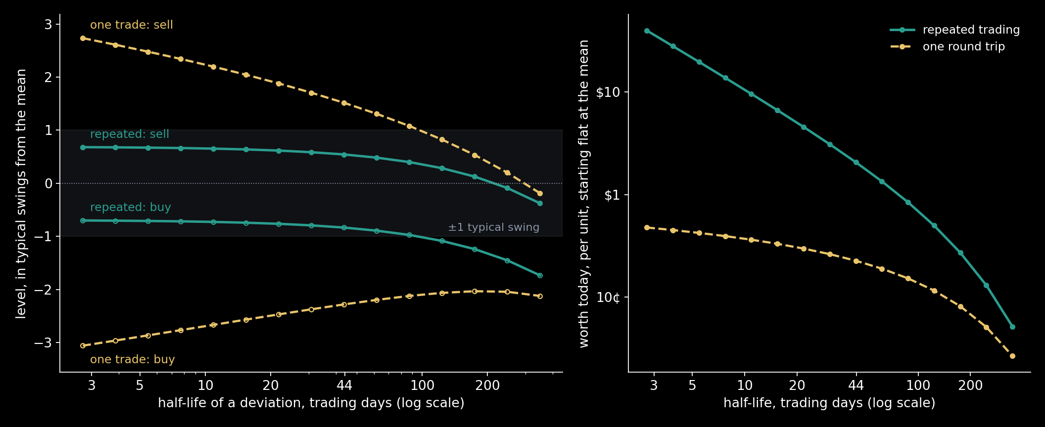
One simulated path of the example price over five years (1,260 trading days). Teal: the repeated-trading levels, 91.7 and 105.4 cents, and its trades (▲ buy, ▼ sell): five round trips. Amber: the one-trade levels, 77.2 and 115.2 cents; that rule bought once, on day 1,164 (the circle), and was still… — **Figure 4.** One simulated path of the example price over five years (1,260 trading days). Teal: the repeated-trading levels, 91.7 and 105.4 cents, and its trades (▲ buy, ▼ sell): five round trips. Amber: the one-trade levels, 77.2 and 115.2 cents; that rule bought once, on day 1,164 (the circle), and was still waiting to sell at the end.

As the price reverts faster, the two rules part company. With a 175-day half-life the one-trade rule buys 2.03 swings down and sells 0.53 up, while repeated trading buys 1.24 down and sells 0.13 up. At 11 days the one-trade levels spread to 2.66 down and 2.20 up; the repeated levels are 0.73 down and 0.65 up. At 3.4 days, 3.00 and 2.66 against 0.70 and 0.68. The repeated band changes little; the trader simply trades more often, 4.3 round trips a year at 11 days and 13.8 at 3.4 days, and the strategy is worth more: $9.59 and $32.21, against 36.3 and 46.1 cents for a single trade.

Left: the buy and sell levels of the two rules against the half-life of a deviation, at a cost of a cent each way, in typical swings from the mean. As reversion gets faster the one-trade rule (amber) waits for ever more extreme prices, while the repeated rule (teal) changes little. Right: what each… — **Figure 5.** Left: the buy and sell levels of the two rules against the half-life of a deviation, at a cost of a cent each way, in typical swings from the mean. As reversion gets faster the one-trade rule (amber) waits for ever more extreme prices, while the repeated rule (teal) changes little. Right: what each rule is worth today, per unit, starting flat at the mean.

Why the Band Sits Below the Mean

The repeated band is lopsided: 0.83 swings below the mean, but only 0.54 above. The reason is the 5%. The price pays no interest, and the money tied up in it could earn $r$. Holding a unit at price $x$ earns the pull toward the mean, $\kappa(\theta – x)$, and gives up the interest, $r\,x$. The two balance at

$$x^{*} = \frac{\kappa\,\theta}{\kappa + r}$$

$(7)$

which for the example is 98.8 cents. The middle of the repeated band is 98.6 cents. This is an observation, measured on the board below, not a theorem: for every half-life up to two months and every cost up to a cent, the middle of the band lies within 0.21 cents of $x^{*}$. For slower reversion and dearer trading the band sits lower still, by up to 4.5 cents.

Try It

The board solves nothing. It looks up a table of 15 half-lives, from 2.7 to 247 trading days, and 6 costs, from a quarter of a cent to 4 cents, each solved by the method above and checked against its own grid; the largest gap anywhere is 0.025 cents. Every card on the board was read back in a browser and compared with Python’s numbers.

Optimal entry and exit for a price that reverts to a dollar with a typical swing of 10 cents. The sliders set how fast it comes back and what a trade costs. The bell is where the price spends its time; teal is repeated trading, amber the single round trip. The cards give the levels, how often a round trip comes, how long the single trade waits for its first purchase, and what each is worth today.

So, Should You Wait?

It depends on one property of the price: whether it comes back.

For a market that drifts up, no. Buy at once. Every waiting rule loses on average, and since 1990 waiting for a 10% dip lost seven times in ten as well. The theorem says nothing about risk: an investor who could not sit through a large fall should own less, not wait.

For a price that comes back, yes, but not as long as the textbook answer for a single trade says. In the example the single trade waits for 77 cents and more than four years; a trader who keeps trading buys at 92 cents, about once a year, and ends up with nine times the value. Patience is priced by the trades you are not making.

The second half rests on assumed numbers. A real spread can stop reverting, through a merger, a delisting or a change in how the market prices it, which is why Leung and Li add a stop-loss. A reversion speed estimated from data is noisy, and a real cost is more than a commission. The first half rests on one market and 36 years of overlapping windows. The theorem underneath it rests on neither.

Sources

R. J. Shiller, monthly stock market data: S&P Composite price, dividends and the 10-year Treasury yield, 1871 to the present (ie_data.xls), shillerdata.com.
G. E. Uhlenbeck and L. S. Ornstein, “On the theory of the Brownian motion”, Physical Review 36 (1930) 823–841.
T. Leung and X. Li, “Optimal mean reversion trading with transaction costs and stop-loss exit”, International Journal of Theoretical and Applied Finance 18 (2015) 1550020.
T. Leung and X. Li, Optimal Mean Reversion Trading: Mathematical Analysis and Practical Applications, World Scientific, Singapore, 2016.
M. Zervos, T. C. Johnson and F. Alazemi, “Buy-low and sell-high investment strategies”, Mathematical Finance 23 (2013) 560–578.

Every number in the text, the charts and the board are computed by the scripts archived with this post: the simulation and the S&P replay from Shiller’s data, and the two trading problems solved once, each checked against a finite-difference grid and a simulation of the rule.

Interested in applying these ideas to your work? Get in touch.