
What a Stop-Loss Costs
The Order Everyone Is Told to Place
Almost every trading book says it: always use a stop-loss. Decide in advance how much you are willing to lose, and let an order sell for you when the price gets there, before hope talks you out of it.
So I tested it on the S&P 500, every month since 1990, with the kind of stop people actually use: sell when the index falls a set amount below its high, buy back when it rises the same amount above its low. With the line drawn at 5%, the stop left investors with a quarter less money five years later. With the line drawn at 10%, it roughly broke even, and it cut the worst fall an investor lived through from 55% to 34%. Same idea, same market; the width of the stop decided everything.

This post is the exit side of the question of when to buy, and it has the same two halves. First a market that drifts upward, where a short argument says what a stop must cost and the real index says something more interesting. Then a price that comes back, where a stop does something stranger: it puts a floor under the price you should buy at, and set too tight, it kills the trade altogether.
The Verdict of a Random Walk
Model the market as a geometric Brownian motion growing at $\mu$ a year, and cash earning $r$. A stop-loss rule decides, from what it has seen so far, whether the money is in the market ($\pi_t = 1$) or in cash ($\pi_t = 0$). Wealth then grows as
and taking expectations, the random part drops out:
If the market beats cash, every day out of the market lowers what you can expect to end with, and no rule that looks only at the past can make that up, because in a random walk the past says nothing about the future. Kathryn Kaminski and Andrew Lo put it in one line in 2014: under the random walk hypothesis, all-or-nothing stop-loss rules always decrease a strategy’s expected return; with momentum, they can add value.
So the real question is not about the stop. It is about the market: does it behave like a random walk at the scale the stop works on?
Four Stops on the S&P 500
I used the daily closes of the S&P 500, with dividends reinvested, and let the money earn the 3-month Treasury bill rate whenever a rule was out of the market. Every month from January 1990 to October 2021 was a start, 382 in all, and each rule was judged five years later against simply holding. The rules:
- A fixed stop: sell when the index closes 10% below the price paid, and buy back when it regains the price sold at.
- Trailing filters of 5%, 10% and 20%: sell when the index closes that far below its highest close since buying, and buy back when it closes that far above its lowest close since selling. These are the filter rules that Eugene Fama and Marshall Blume tested in 1966.
Then I ran the same four rules in a random walk with the index’s own numbers since 1990: growth of 11.9% a year, volatility of 18%, and cash at the average bill rate of 2.7%, over 20,000 simulated five-year paths.
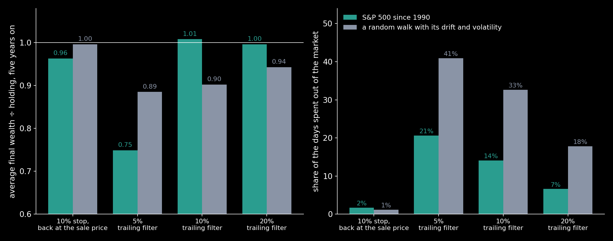
The random walk did exactly what the argument says. Every rule ended behind holding on average: the 10% filter by about 10%, ahead of holding in only a quarter of the paths, and out of the market a third of the time.
The real index split the rules apart. The 5% filter was whipsawed: 34.5 trades in five years on average, out of the market a fifth of the time, ahead of holding in 5% of the starts, and left with 25% less. The 10% filter traded 8 times in five years, was out 14% of the time, and ended with 1.008 times what holding gave: break-even, within the noise. The 20% filter came in at 0.996. With a cost of 0.1% on every trade the 10% filter drops to 0.999.
What the wider stops did buy was protection. The worst fall an investor lived through with the 10% filter, peak to trough inside the five years, was 34%, against 55% for holding, and the worst five-year outcome was 0.84 of the money put in, against 0.67.
The fixed stop is the odd one. It buys back at exactly the price it sold at, so it can never come out ahead of holding by more than the interest earned while out; its best start finished at 1.00. And it can do worse than holding: a stop that buys back at its sale price can sell, buy back on a rebound and ride the next leg down, and its worst fall came out deeper than holding’s, 63% against 55%. It ended at 0.963 on average.
Why did the real market treat the 10% and 20% filters so much better than a random walk with the same volatility? Because its volatility is not the same all the time. In a random walk with 18% a year, a 10% fall from the high comes round often, and the filter keeps stepping out and paying to get back in: out a third of the time. In the real index the calm years rarely fell 10%, so the filter stayed in, and the falls that did trigger it came in runs, in 2000 to 2002 and in 2008, where getting out and staying out paid. That is the kind of departure from a random walk that Kaminski and Lo describe, and the 5% filter shows its other side: in turbulent years, a tight stop is sold and bought back again and again.
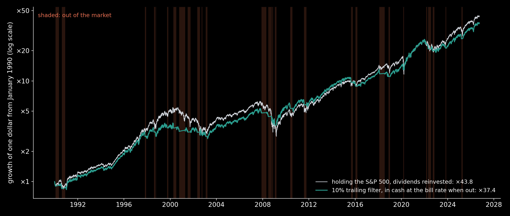
And the window matters. Run continuously from the first trading day of 1990, instead of in five-year pieces, the same 10% filter made 58 trades and turned a dollar into 37.4, against 43.8 for holding: about 15% behind. Averaged over five-year windows it broke even; over 36 years in one piece it lost to holding.
Three cautions belong next to these numbers. I tested four widths, and the one that looks best is the one I would have picked only in hindsight: that is exactly the kind of result that fails to repeat. The 382 starts overlap, so 36 years hold only about seven independent five-year windows, and two crashes do most of the work. And taxes, which fall on every sale in a taxable account, are not counted at all.
A Price That Comes Back, With a Stop
For a price that reverts to a level, a stop-loss means something else. Take the price from the earlier post: it reverts to $1.00 with a typical swing of 10 cents and a half-life of 44 trading days, a trade costs a cent each way, money is worth 5% a year, and one unit is held at a time; all assumed. Without a stop, the best single trade buys at 77.2 cents and sells at 115.2, and repeated trading buys at 91.7 and sells at 105.4.
Now add a stop at $L$: a long position is sold the moment the price touches it. Tim Leung and Xin Li solved the single trade with a stop in 2015. With $\tau_L$ the first time the price falls to $L$, the exit and the entry become
and between its levels the value is again built from the two solutions $F$ and $G$ of $(\mathscr{L} – r)f = 0$, the increasing and the decreasing one, that solved the earlier post’s problems.

The Falling Knife, Derived
Without a stop, the rule was: buy once the price falls to a level, and the lower the better. With a stop, the answer changes shape. The buy region becomes a band, bounded below as well as above. Below the band the price is too cheap to buy, because it is too close to where the stop would sell it at a loss before it has had time to come back. “Never catch a falling knife” stops being a proverb and becomes the lower edge of a solved problem.
For the single trade, with the stop at 70 cents, the band runs from 78.6 to 80.7 cents and the trade is worth 16.3 cents today, starting flat at the mean, against 22.6 without a stop. With the stop at 75 cents the band is 83.5 to 84.2 cents and the trade is worth 10.0 cents. At 80 cents the band has shrunk to 87.64 to 87.89 cents, a quarter of a cent wide, and the trade is worth 4.1 cents. At 85 cents it is two hundredths of a cent wide, at 91.18 to 91.20, and worth 0.4 of a cent. From 86 cents, 1.4 typical swings below the mean, there is no band at all: no single trade is worth taking.
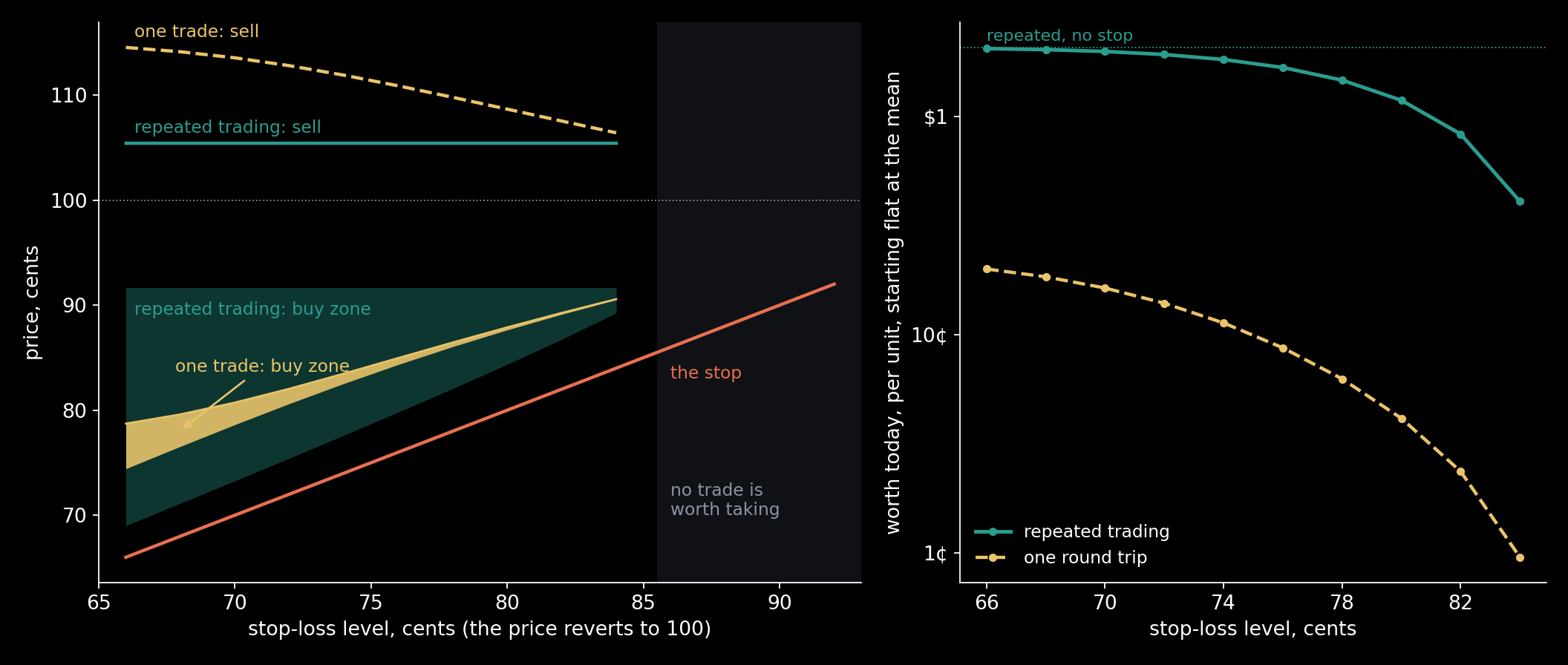
I checked the single trade the same three ways as before. With the stop at 80 cents a finite-difference grid that treats the stop as a forced sale and uses no formula puts the band at 87.64 to 87.88 cents and the sale at 108.64, against 108.66 from the closed form. A simulation of the rule itself gives 4.22 ± 0.19 cents for the trade’s value.
Trading It Again and Again
The lesson of the earlier post was that a trader who keeps trading should not use the single-trade answer, and the same holds with a stop. Repeated trading with a stop is a problem I have not found in the literature, so I solved it. Being long is worth $V$, being flat is worth $J$, and a stop-out sends the position straight back to flat. With $V = B_1F + B_2G$ between the stop and the sale level $b$, and $J = A_1F$ below the floor $a$ and $A_2G$ above the top $d$ of the buy zone, value matching and smooth fit give seven conditions for the seven unknowns:
With the stop at 80 cents, repeated trading buys anywhere between 84.4 and 91.7 cents and sells at 105.4, and the whole strategy is worth $1.18 today, against $2.07 without the stop. The top of the zone and the sale level do not move at all; the stop only adds the floor, and the floor rises with it: 73.3 cents for a stop at 70, 78.7 for a stop at 75, 90.6 for a stop at 85. From 86 cents, again, no trade is worth taking.
How often does the stop fire? The chance that a purchase ends at the stop rather than at the target comes from the scale function of the process, $S^{\prime}(x) = e^{\kappa(x-\theta)^2/\sigma^2}$:
The second line holds because a purchase at the top of the zone follows a sale at the target, and a purchase at the floor follows a stop-out. With the stop at 80 cents, 28.5% of the trades bought at the top end at the stop, and 58.4% of those bought at the floor, so in the long run 40.7% of all trades end at the stop. The simulation counts 40.7% too.
Algorithm — Repeated Trading of a Reverting Price With a Stop-Loss
input:  κ, θ, σ, r, the cost c each way, the stop L
F, G ← the increasing and decreasing solutions of (𝓛 − r) f = 0
grid ← 4,001 prices over ±8 typical swings, upwind differences
    the stop as a forced sale; policy iteration on V and J
seed ← the grid's levels a, d, b and values (a starting point only)
(B₁, B₂, A₁, A₂, a, d, b) ← the seven conditions, solved exactly
check: the levels against the grid, to a grid step
check: the rule itself, 20,000 paths, 4 steps a day, 40 years,
    a Brownian-bridge test for a level touched between steps,
    open positions valued at the end
share at the stop ← p(d) / (1 − p(a) + p(d)), from the scale
    function; checked against the simulation's count
The grid agrees at every stop: with the stop at 80 cents it puts the zone at 84.36 to 91.68 cents and the strategy at $1.181, and the simulation gives $1.180 ± 0.006.
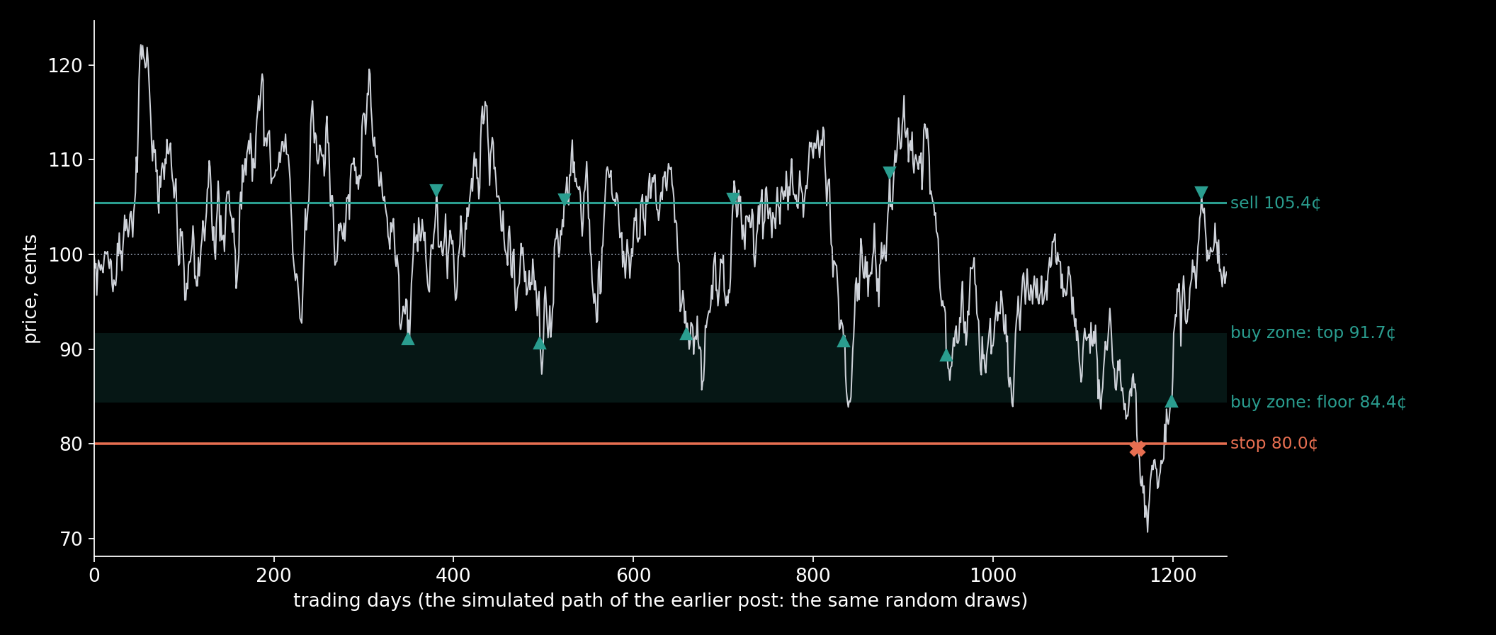
On that path the stop did what stops do. The position bought on day 948 at the top of the zone rode the dip down, was sold at 80 cents on day 1,161, eleven days before the price bottomed at 70.7 cents, and the rule bought back on day 1,199 at the floor. Without the stop the same position would have been held through the whole dip and sold at 105.4 on day 1,232, the same day the stopped trader sold.
Try It
The board looks up a table of 5 half-lives, from 11 to 175 trading days, and 15 stops, from none to 92 cents, each solved by the method above and checked against its own grid; the largest gap anywhere is 0.03 cents. Every card was read back in a browser and compared with Python’s numbers.
So What Does a Stop Cost?
In a random walk, a stop costs money, always: every day out of the market is a day of growth given up, and the past cannot tell you which days to skip.
On the real S&P 500 since 1990, the cost depended on the width of the stop. A tight one was a heavy fee; a wide one roughly paid for itself in five-year windows and took the edge off the worst falls, though over 36 years in one piece it still trailed holding. Before choosing a stop from a table like this one, remember that the best row is visible only afterwards.
For a price that comes back, a stop costs value and changes where you should buy. It draws a floor under the buy zone, the falling knife made precise, and the tighter it is, the higher the floor, until, with the stop 1.4 typical swings below the mean, no trade is worth taking at all.
Sources
- K. M. Kaminski and A. W. Lo, “When do stop-loss rules stop losses?”, Journal of Financial Markets 18 (2014) 234–254.
- paveljurke, “S&P 500 (^GSPC) Historical Data”, Kaggle dataset (CC0), daily closes from Yahoo Finance.
- R. J. Shiller, monthly stock market data: S&P Composite price, dividends and the 10-year Treasury yield, 1871 to the present (ie_data.xls), shillerdata.com.
- Board of Governors of the Federal Reserve System, 3-Month Treasury Bill Secondary Market Rate (DTB3), retrieved from FRED, Federal Reserve Bank of St. Louis.
- E. F. Fama and M. E. Blume, “Filter rules and stock-market trading”, The Journal of Business 39 (1966) 226–241.
- G. E. Uhlenbeck and L. S. Ornstein, “On the theory of the Brownian motion”, Physical Review 36 (1930) 823–841.
- T. Leung and X. Li, “Optimal mean reversion trading with transaction costs and stop-loss exit”, International Journal of Theoretical and Applied Finance 18 (2015) 1550020.
- M. Zervos, T. C. Johnson and F. Alazemi, “Buy-low and sell-high investment strategies”, Mathematical Finance 23 (2013) 560–578.
Every number in the text, the charts and the board are computed by the scripts archived with this post: the stop-loss rules on daily S&P 500 data and in a random walk, and the two trading problems with a stop, each checked against a finite-difference grid and a simulation of the rule.
Interested in applying these ideas to your work? Get in touch.