The Wave That Nobody Ordered

Four Cases, Then Eight

For more than sixty years, students and executives at MIT and far beyond have sat down in teams of four to play a board game about beer. One plays a retailer, one a wholesaler, one a distributor and one a brewery. Customers buy beer from the retailer, who orders from the wholesaler, who orders from the distributor, who orders from the factory. Nobody may talk to anybody else. Each player sees one thing: the orders that arrive from the next player down the chain.

The customers are a deck of cards. For four weeks they buy 4 cases a week. In week 5 they buy 8, and they go on buying exactly 8, week after week, until the game ends.

After the game, the players are asked to sketch what the customers did. In John Sterman’s experiments at MIT, the majority draw a surge: demand climbing from 4 to a peak of anywhere between 12 and 40 cases a week, then collapsing towards nothing. When the deck of cards is turned over and they see the single step from 4 to 8, many are shocked; some, Sterman writes, “voice strong disbelief”.

A brewery cellar. At the far end of a supply chain, the factory sees the customers only through three other people's orders. — **Figure 1.** A brewery cellar. At the far end of a supply chain, the factory sees the customers only through three other people’s orders.

A Board of Stocks and Flows

The game is slow on purpose. An order spends 2 weeks in the mail before the supplier reads it, and the beer then spends 2 weeks on the road. The factory’s requests take a week to reach the brewhouse and the brewing takes 2 more. Every station starts with 12 cases, every delay holds 4, and every case costs its holder 50 cents a week to keep, while every case owed to a customer and not yet delivered costs a dollar a week.

That makes it a system of stocks and flows, the language Jay Forrester invented at MIT for exactly this kind of problem. Each station has an inventory, a backlog of orders it could not fill, and an expectation of demand:

$$\begin{aligned} \frac{d\,\mathrm{INV}_i}{dt} &= \text{arrivals}_i – \text{ship}_i \\[2pt] \frac{d\,\mathrm{BL}_i}{dt} &= \text{incoming}_i – \text{ship}_i \\[2pt] \frac{dE_i}{dt} &= \theta\,(\text{incoming}_i – E_i) \end{aligned}$$

$(1)$

The one decision in the game is how much to order. In 1989 Sterman proposed a rule that people plausibly follow, the one anyone would describe in words: order what you expect to sell, plus part of the gap between the stock you want and the stock you have, plus part of the gap between the beer you want on its way and the beer that is actually on its way:

$$\begin{aligned} O_i = \max\big(0,\ & E_i + \alpha_S\,(S^* – \mathrm{INV}_i + \mathrm{BL}_i) \\ & + \alpha_S\,\beta\,(\hat\lambda\,E_i – \mathrm{SL}_i)\big) \end{aligned}$$

$(2)$

$\mathrm{SL}_i$ is the supply line: everything the station has ordered and not yet received. $\alpha_S$ is how much of the stock gap it closes each week, $S^*$ the stock it wants, $\hat\lambda$ the lead time it believes in, and $\theta$ how quickly its forecast follows the orders it sees. And $\beta$ is the share of the supply line it takes into account: 1 counts everything already ordered, 0 forgets it the moment the order slip leaves the table.

Sterman then fitted the rule to each of 44 real players. On average they closed a quarter of their stock gap each week ($\alpha_S = 0.26$) and moved their forecast about a third of the way towards each week’s orders ($\theta = 0.36$). And they counted about a third of the beer already on its way to them: $\beta = 0.34$. Only five of the 44 counted more than two thirds of it. They also allowed for too little beer in the pipeline: 8.4 cases where 16 were needed, as if the beer took about 2 weeks to come instead of 4.

The Board, Running

I wrote the game in the style the industry calls system dynamics: everything that accumulates is a stock, every rate that fills or drains a stock is a flow, and the model is the set of ordinary differential equations that ties them together. Each delay box of the board becomes a stock that empties at its contents divided by its delay, so a 2-week delay is two 1-week boxes in a row, and the whole chain is 27 equations:

Algorithm — Thirty-Six Weeks of Beer

input:  4 stations: retailer, wholesaler, distributor, factory
        each starts with 12 cases; every delay box holds 4
        customers buy 4 cases a week; from week 5 on, 8
        delays: orders 2 weeks in the mail, beer 2 weeks on the road
                (the factory: 1 week for requests, 2 for brewing)
        the rule: θ, α_S, β, S* and λ (the lead time the player
                  believes), the same at every station

y <- 27 stocks: each station's inventory, backlog and forecast,
     two boxes for every delay, and the factory's three

repeat for 36 weeks, in steps of dt = 1/32 week:
    for every station:
        incoming <- the customers, or the orders leaving the mail
        ship     <- min(incoming + backlog / τf, inventory / τf)
                                        τf = 1/8 week: ship what you have
        SL       <- its mail boxes + the supplier's backlog
                    + its boxes on the road
        order    <- max(0, E + α_S (S* − inventory + backlog)
                              + α_S β (λ E − SL))     (weeks 1–4: 4)
    every box: d(contents)/dt = what flows in − contents / its delay
    advance all 27 stocks by one Runge–Kutta step (RK4)
    each station pays dt × ($0.50 × inventory + $1 × backlog)

search: 7,200 rules on a grid of θ, α_S, β, S* and λ;
        keep the one with the cheapest team

The board below solves the same equations in your browser, every time you move a slider:

The Beer Game as a board of stocks and flows. Each station has a red backlog box and a tall inventory box; orders travel up the chain in amber, two boxes in the mail, and beer travels down it in blue, two boxes on the road, with every valve showing its rate. Press run to play the 36 weeks from the start: the charts draw themselves as the weeks pass, and the diamonds mark where the real teams' orders peaked on average. The sliders change how every player orders and the world they order in, and the board re-solves at once; the presets load the players' average rule, the same players counting everything already ordered, and the cheapest rule found. The last chart runs the whole game again for 21 values of β at your settings. Below the board: the model.

A Third of the Pipeline

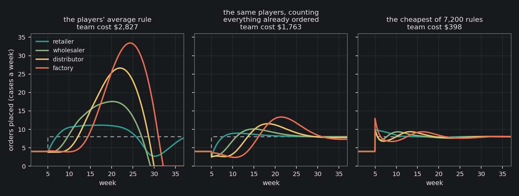
Fed the players’ average rule, the model does what the real teams did. The retailer’s orders rise to 11 cases a week, the wholesaler’s to 18, the distributor’s to 27, and the factory’s to 33, each peak later than the one before. Sterman’s real teams averaged 15, 19, 27 and 32. One step of 4 cases in customer demand becomes a swing of 29 at the brewery: an amplification of 7.4 times in the model, 7 times in the real games.

The mechanism fits in a sentence. A player who has run short orders more, and keeps ordering more every week the shelves stay empty, because two thirds of what they have already ordered has slipped out of mind; four weeks later it all arrives at once. The supplier, who saw those orders, has done the same a step further up.

It is expensive. Over 36 weeks the players’ rule costs the team $2,827, against $398 for the cheapest rule I found: 7.1 times as much. The real teams paid 9.9 times the benchmark Sterman computed.

Counting What Is Already on Its Way

Now change one number. Let the same players count everything already ordered, $\beta = 1$, and leave the rest alone. The factory’s peak falls from 33 cases a week to 13, and the team’s bill from $2,827 to $1,763.

That is not the whole cure, because the second misperception is still there: players who believe the beer takes 2 weeks keep half the pipeline they need. At first the stations up the chain even order less than 4, because the pipeline they count looks too full. Fix that too, give them the true lead time of 4 weeks, and the bill falls to $1,275; but the factory still swings 4 times harder than the customers, because a forecast that chases every change in orders passes each ripple on.

The cheapest of the 7,200 rules does not chase at all ($\theta = 0$). It closes the whole stock gap every week, counts three quarters of its supply line and allows for 6 weeks of pipeline. It reacts at once: every station’s orders jump in week 5, the factory’s to 13 cases, and then settle. Nobody ever runs deeply short, and the team pays $398. It is close to the benchmark rule Sterman computed in 1989.

The same step in customer demand (dashed), three ways of ordering. Left: the players' average rule; the factory's orders peak at 33 cases a week. Middle: the same players counting everything already ordered; 13. Right: the cheapest of 7,200 rules, which reacts at once instead of late. — **Figure 2.** The same step in customer demand (dashed), three ways of ordering. Left: the players’ average rule; the factory’s orders peak at 33 cases a week. Middle: the same players counting everything already ordered; 13. Right: the cheapest of 7,200 rules, which reacts at once instead of late.

The Diapers

The game is not a curiosity. Logistics executives at Procter & Gamble once looked at the orders for Pampers. Babies use diapers at a steady rate, and the shops’ sales moved only a little; yet the distributors’ orders to P&G swung harder than the shops’ sales, and P&G’s own orders to its suppliers swung harder still. They called it the bullwhip effect. In 1997 Hau Lee, V. Padmanabhan and Seungjin Whang told that story and showed how the effect grows out of sensible decisions inside the structure of the chain, without anyone behaving badly.

**Figure 3.** Waves growing as they run in towards a harbour wall. A supply chain does to one step in demand what a shelving shore does to a swell.

Blaming the Customers

The most telling part of the game is what happens afterwards. Asked to explain the chaos, most players blame the customers, who seemed to want more and more beer and then suddenly none. Few ever say: I ordered too much because I forgot what I had already ordered. The waves came from inside the chain, from four people each following a sensible rule with a hole in it, and every one of them saw the waves arriving from outside.

That is why better forecasting is the wrong cure. Sterman put it in one line: “Even a perfect forecast will not prevent a manager who ignores the supply line from overordering.”

**Figure 4.** An empty shop shelf. The shortage and the glut that follows it are the same wave, seen at two moments.

The customers in the Beer Game changed their minds once, from 4 cases a week to 8, and never again. The wave that went up the chain, 11 then 18 then 27 then 33, was ordered by nobody, and it was built from the one number every player could have counted: what was already on its way.

Sources

J. D. Sterman, “Modeling managerial behavior: misperceptions of feedback in a dynamic decision making experiment”, Management Science 35 (1989) 321–339.
J. W. Forrester, Industrial Dynamics (1961).
H. L. Lee, V. Padmanabhan and S. Whang, “The bullwhip effect in supply chains”, Sloan Management Review 38 (1997) 93–102.

The model, the 7,200-rule search and every number from the model in the text are computed by the scripts archived with this post, from results saved once; the real teams’ numbers are Sterman’s.

Interested in applying these ideas to your work? Get in touch.