Markov Chains in Supermarket Management

The Supermarket as a Stochastic System

A supermarket is full of queues, decisions, and uncertainty. Customers arrive unpredictably, spend varying amounts of time at different sections, and leave when they are done. Managing the operation — how many checkout lanes to open, where to place high-margin products, when to reorder stock — requires a model of how people and inventory move through states over time.

Markov chains are that model. The Markov property is simple: the probability of what happens next depends only on the current state, not on the history of how you got there. A queue with four people in it behaves the same way whether it built up quickly or slowly. This is often a good approximation in retail — and it leads to surprisingly clean results.

Managing the Checkout Queue

The checkout queue is the most natural application. Model it as a **birth-death chain**: the state is the number of customers currently in the system (queuing plus being served). Customers arrive at rate $\lambda$ — on average, $\lambda$ arrivals per minute. Each cashier serves customers at rate $\mu$. With $c$ cashiers open, the system is an M/M/c queue.

The transitions are simple:

$$\lambda_n = \lambda, \qquad \mu_n = \min(n, c)\,\mu$$

$(1)$

From state $n$, the queue grows to $n+1$ at rate $\lambda$ (a new arrival) or shrinks to $n-1$ at rate $\min(n,c)\mu$ (a service completion). The **traffic intensity** $\rho = \lambda / (c\mu)$ measures how loaded the system is. If $\rho < 1$, the queue is stable — customers are served faster than they arrive on average. If $\rho \geq 1$, the queue grows without bound.

The stationary distribution — the long-run probability of being in state $n$ — gives the full picture. For a single cashier (M/M/1), it has a clean closed form:

$$\pi_n = (1 – \rho)\,\rho^n$$

$(2)$

This is a geometric distribution in the queue length. The mean queue length is $\rho / (1 – \rho)$: at 50% load the average queue has one person; at 90% load it has nine. The deterioration is nonlinear — a system that runs fine at 70% load becomes chaotic at 90%.

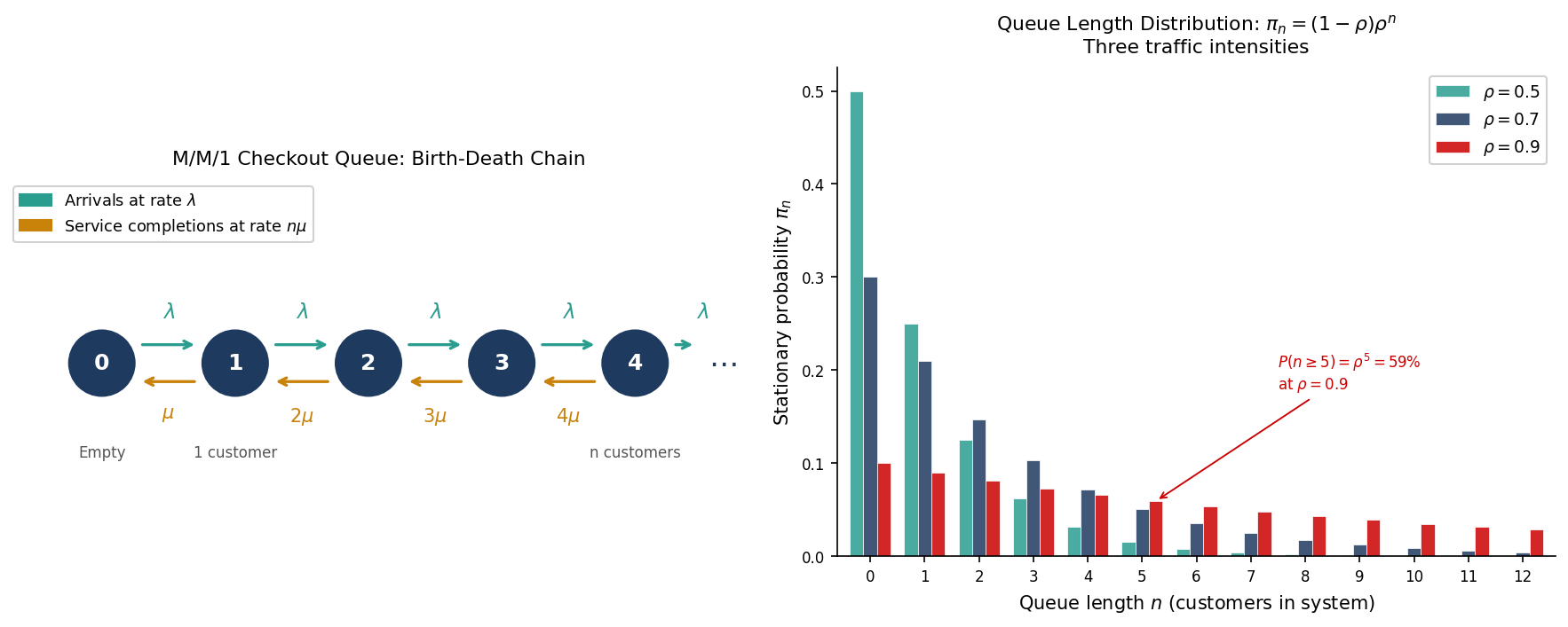
**Figure 1.** Left: the birth-death chain structure for the M/M/1 checkout queue. States represent the number of customers in the system; transitions move right at arrival rate $\lambda$ and left at service rate $\mu$. Right: the stationary queue-length distribution $\pi_n = (1-\rho)\rho^n$ for three traffic intensities $\rho = 0.5$, $0.7$, $0.9$. At low load the queue is almost always empty; at $\rho=0.9$ there is a 35% chance of four or more customers waiting.

The practical use is direct. Given arrival rate data (from till timestamps) and average service times, the manager can compute $\rho$ in real time and set a threshold — say, open a new lane whenever $\rho > 0.75$. The stationary distribution quantifies the cost of waiting: the probability that a customer faces a queue of five or more is $\pi_{\geq 5} = \rho^5$. At $\rho = 0.9$, that is 59%. At $\rho = 0.75$, it falls to 24%.

Customer Flow Through the Store

A second application is less obvious but equally useful. Model the store itself as a Markov chain, where the states are sections — produce, dairy, bakery, frozen, checkout — and the transition matrix $P$ captures where customers tend to go next.

From transaction and loyalty card data, the entry $P_{ij}$ can be estimated: the fraction of customers who visit section $i$ and then move directly to section $j$. The **stationary distribution** $\pi$ of this chain tells you where customers spend the most time on average.

This has direct implications for layout. Sections with high stationary probability are high-traffic — placing impulse-purchase items there increases exposure. Sections with low transition probability from high-traffic areas represent dead zones: customers rarely continue there, so stocking them with staple necessities (milk, bread) draws foot traffic deeper into the store.

The same framework identifies **bottlenecks**: sections where the chain gets “stuck”, with high self-transition probability $P_{ii}$. These are either engaging (a well-merchandised bakery) or frustrating (a confusing frozen foods layout). The data distinguishes the two by correlating dwell time with basket value in that section.

What Markov Chains Cannot Do

The Markov property assumes the next step depends only on where you are now — not on how long you have been there, or where you came from. This is a simplification. A customer who has been in the frozen aisle for five minutes probably behaves differently from one who just arrived. A queue that spiked due to a promotion arrival pattern differs from steady-state traffic.

Extensions exist — semi-Markov processes allow state-dependent holding times, hidden Markov models account for unobserved customer types — but the basic chain is often sufficient for operational decisions. The model does not need to be perfect to be useful. A manager who knows that running at $\rho = 0.85$ means a one-in-three chance of a queue exceeding six people has actionable information, even if the true arrival process is not Poisson.

The supermarket is a useful reminder that Markov chains are not an abstract tool. They are a direct description of how systems move between states under uncertainty — which is exactly what a retail operation is.

Interested in applying these ideas to your work? Get in touch.