The Return That Takes Four Centuries

Two Numbers

Everyone who owns a share would like to know two numbers about it: how much it returns on average, and how much it
swings. The two sound equally hard to measure. They are not. Take a share whose price swings by 20% a year and whose
expected return is 5% a year. One day of prices sampled every minute tells you its volatility to within 0.72 of a
percentage point. To learn its expected return to within one percentage point, you need 400 years of prices.

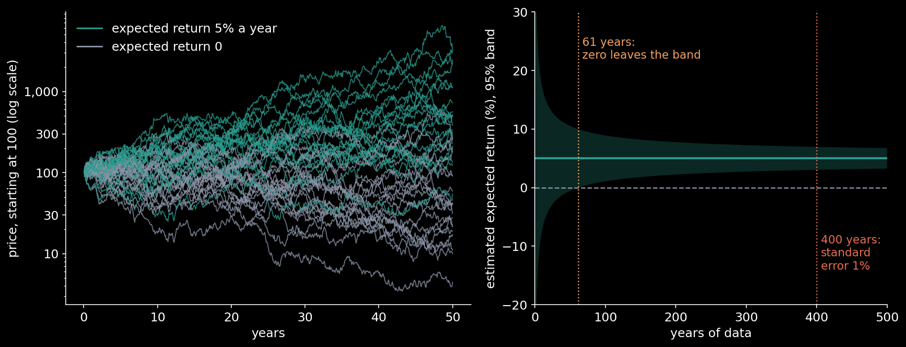
With fifty years of data, a lifetime of saving, the best estimate of that 5% comes with a 95% band of plus or minus 5.5
points: it cannot even tell the share apart from one that returns nothing. It takes 61 years before zero drops out of the
band. The volatility, meanwhile, was known on the first morning.

**Figure 1.** Prices on a trading screen: every wiggle in them measures the volatility, and none of them measures the expected return. Photograph by Alesia Kozik, Pexels.

The Wiggle and the Trend

The standard model of a share price $S_t$ is geometric Brownian motion, and its logarithm $X_t = \ln S_t$ is a Brownian
motion with a drift:

$$\frac{dS_t}{S_t} = \mu\,dt + \sigma\,dW_t, \qquad X_T – X_0 = \nu T + \sigma W_T, \qquad \nu = \mu – \tfrac12\sigma^2$$

$(1)$

Here $\mu$ is the expected return, $\sigma$ the volatility and $W$ a standard Brownian motion. Every return the share
ever makes is a small piece of $\nu T + \sigma W_T$: a trend that grows with time and a wiggle that grows with its square
root. Over a year the trend is 5 points and the wiggle 20. Over a day the trend is two hundredths of a point and the
wiggle more than one point. The shorter the interval, the more completely the wiggle drowns the trend.

What a Century Cannot Tell

Suppose you observe the log price at $n$ equally spaced times over $T$ years and estimate the drift the obvious way, by
averaging the returns. The sum of the returns telescopes:

$$\hat\nu = \frac{1}{T}\sum_{i=1}^{n}\big(X_{t_i} – X_{t_{i-1}}\big) = \frac{X_T – X_0}{T}, \qquad \operatorname{sd}(\hat\nu) = \frac{\sigma}{\sqrt T}$$

$(2)$

Every price between the first and the last cancels out. This average is also the maximum-likelihood estimate, so no
cleverer use of the same prices does better. The precision depends on one thing only, the length of the record: 6.3
points of standard error over ten years, 2.8 over fifty, 2.0 over a century. At 20% volatility, a standard error of one
point needs $(0.20/0.01)^2 = 400$ years. And the estimate is noisy enough to mislead outright: in a simulation of 20,000
fifty-year histories of a share that truly returns 5% a year, 4.0% of them show a negative average return; the formula
says 3.9%.

Left: twenty fifty-year price histories of a share returning 5% a year (teal) and twenty of a share returning nothing (grey), driven by the same random shocks; by eye they cannot be told apart. Right: the 95% band of the expected return estimated from a record of each length. Zero leaves the band… — **Figure 2.** Left: twenty fifty-year price histories of a share returning 5% a year (teal) and twenty of a share returning nothing (grey), driven by the same random shocks; by eye they cannot be told apart. Right: the 95% band of the expected return estimated from a record of each length. Zero leaves the band after 61 years; the standard error falls to one point only after 400.

What a Day Can Tell

Volatility is the opposite. Square the returns instead of adding them, and the sum converges, as the sampling gets finer,
to a quantity that depends on the volatility alone. This is the quadratic variation of the path, which Paul Lévy showed
is exactly $\sigma^2 T$ for every path of a Brownian motion, with no randomness left:

$$\sum_{i=1}^{n}\big(X_{t_i} – X_{t_{i-1}}\big)^2 \ \longrightarrow\ \sigma^2 T \quad (n \to \infty), \qquad \operatorname{sd}(\hat\sigma) \approx \frac{\sigma}{\sqrt{2n}}$$

$(3)$

The drift contributes to each squared return only at the order of the square of the time step, and disappears. The
precision now depends on the number of returns and not on the length of the window. One trading day of one-minute returns
is 390 returns, enough to know a 20% volatility to 0.72 of a point; the simulation gives 0.71. A whole year of daily
closing prices, 252 returns, does slightly worse, at 0.89. The day beats the year.

This is the code that checks it. It estimates both numbers from simulated prices, the drift from the first and the last
price and the volatility from the squared returns, and prints what the text above states:

Python 3.13 — Expected Return and Volatility From One Price Series

import numpy as np

mu, sigma = 0.05, 0.20                   # expected return and volatility, per year
nu = mu - sigma**2 / 2                   # drift of the log price: 3%
rng = np.random.default_rng(20260930)

def log_returns(histories, years, per_year):
    """simulated log returns, one row per price history"""
    dt = 1 / per_year
    return rng.standard_normal((histories, round(years * per_year))) * sigma * np.sqrt(dt) + nu * dt

def estimate(dX, T):
    """log returns over T years -> expected return, its error, volatility, its error"""
    nu_hat = dX.sum(axis=-1) / T                   # only the first and the last price enter
    sig_hat = np.sqrt((dX**2).sum(axis=-1) / T)    # the path's own wiggle
    n = dX.shape[-1]
    return nu_hat + sig_hat**2 / 2, sig_hat / np.sqrt(T), sig_hat, sig_hat / np.sqrt(2 * n)

# the expected return: its error falls with the years watched, never with how often
for T in (10, 50, 100, 400):
    print(f"{T} years: expected return to ±{sigma / np.sqrt(T):.2%}")
print(f"zero leaves the 95% band after {(1.96 * sigma / mu)**2:.0f} years")
for histories, per_year, name in ((20_000, 12, "monthly"), (4_000, 252, "daily")):
    mu_hat = estimate(log_returns(histories, 50, per_year), 50)[0]
    print(f"{histories:,} histories of 50 years, {name}: spread {mu_hat.std():.2%}, below zero {np.mean(mu_hat < 0):.1%}")

# the volatility: its error falls with the number of returns, never with the window
for n, T, name in ((390, 1/252, "one day, every minute"), (252, 1, "one year, daily"), (78, 1/252, "one day, every 5 minutes")):
    sig_hat = estimate(log_returns(20_000, T, n / T), T)[2]
    print(f"{name}: volatility to ±{100 * sigma / np.sqrt(2 * n):.2f} points, simulated {100 * sig_hat.std():.2f}")

# 10 years: expected return to ±6.32%
# 50 years: expected return to ±2.83%
# 100 years: expected return to ±2.00%
# 400 years: expected return to ±1.00%
# zero leaves the 95% band after 61 years
# 20,000 histories of 50 years, monthly: spread 2.86%, below zero 4.0%
# 4,000 histories of 50 years, daily: spread 2.87%, below zero 3.5%
# one day, every minute: volatility to ±0.72 points, simulated 0.71
# one year, daily: volatility to ±0.89 points, simulated 0.89
# one day, every 5 minutes: volatility to ±1.60 points, simulated 1.59

Why the Path Keeps One Secret

The deeper reason is a theorem of Igor Girsanov. Two Brownian motions with the same volatility and different drifts have
laws that are equivalent over any finite time: one is obtained from the other by reweighting the paths,

$$\frac{d\mathbb P_\nu}{d\mathbb P_0}\bigg|_{[0,T]} = \exp\!\Big(\frac{\nu}{\sigma}W_T – \frac{\nu^2}{2\sigma^2}\,T\Big),$$

$(4)$

a density that is strictly positive on every path. Every history that can happen with a 5% drift can happen with a zero
drift, only a little more or less often; no finite record can rule either out. Two volatilities are different: the laws of
Brownian motions with $\sigma$ and $\sigma^{\prime}$ give their paths different quadratic variations with certainty, so they live on
disjoint sets of paths and a single path decides between them.

This is also why the Black–Scholes formula contains the volatility and not the expected return. Pricing an option changes
the drift of the share by exactly the reweighting above, which is allowed because it changes no path’s possibility. The
part of the model that the change of measure throws away is the part no history could have measured anyway; the part it
keeps is the part a single day reveals.

What Sampling Buys

So sampling more often buys everything for the volatility and nothing at all for the expected return. The same fifty years
of data, read monthly or daily, give the same estimate of the drift to the last decimal, because only the first and the
last price enter; read every minute, the volatility is pinned down within a morning.

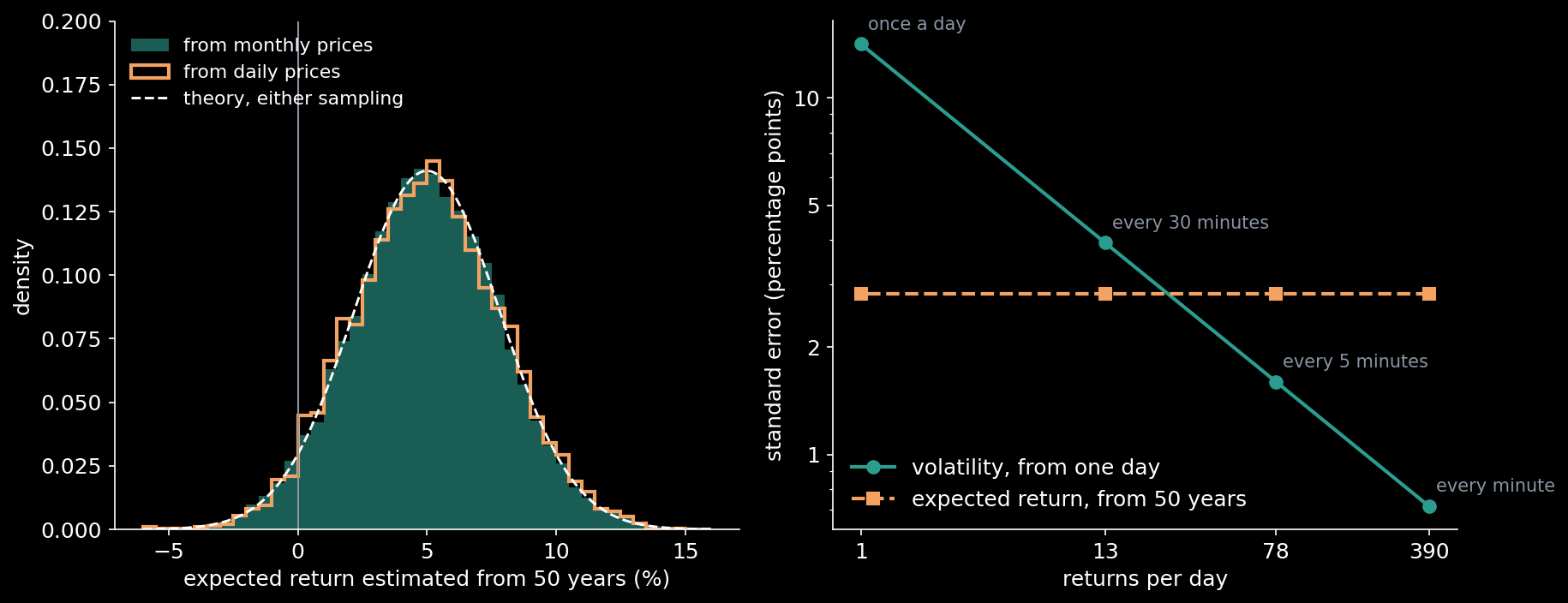
Left: the expected return estimated from fifty years of monthly prices (teal) and of daily prices (orange), each over thousands of simulated histories, against the theory for both (dashed): thirty times more data, no gain. Right: the standard error of the volatility estimated from one day (teal)… — **Figure 3.** Left: the expected return estimated from fifty years of monthly prices (teal) and of daily prices (orange), each over thousands of simulated histories, against the theory for both (dashed): thirty times more data, no gain. Right: the standard error of the volatility estimated from one day (teal) falls with every extra return, while that of the expected return estimated from fifty years (orange) does not move.

Real markets add two caveats, and neither rescues the drift. At very high frequency the recorded prices bounce between
bid and ask, so realised volatility is usually computed from five-minute returns, 78 a day, which still gives a 20%
volatility to 1.6 points. And volatility itself moves, so a day’s realised volatility measures that day’s; that is a
feature, and it is why realised volatility became the workhorse of volatility forecasting. The expected return has no such
workhorse. Robert Merton made the point in 1980: estimating it is a matter of the length of history, and no amount of
data within a history substitutes for more years.

Four Centuries

The Dutch East India Company was founded in Amsterdam in 1602, and its shares were the first to trade on a stock exchange.
That was 424 years ago. A market as old as the oldest one, holding a steady 5% return and 20% volatility all the while,
would only now have told us its expected return to within a percentage point.

**Figure 4.** Amsterdam, where shares were first traded, in 1602. Photograph by Mathias Reding, Pexels.

Its volatility it would have told us on the first day.

Sources

R. C. Merton, “On estimating the expected return on the market: an exploratory investigation”, Journal of Financial Economics 8 (1980) 323–361.
P. Lévy, “Le mouvement brownien plan”, American Journal of Mathematics 62 (1940) 487–550.
I. V. Girsanov, “On transforming a certain class of stochastic processes by absolutely continuous substitution of measures”, Theory of Probability and Its Applications 5 (1960) 285–301.
F. Black and M. Scholes, “The pricing of options and corporate liabilities”, Journal of Political Economy 81 (1973) 637–654.
T. G. Andersen, T. Bollerslev, F. X. Diebold and P. Labys, “Modeling and forecasting realized volatility”, Econometrica 71 (2003) 579–625.
L. Zhang, P. A. Mykland and Y. Aït-Sahalia, “A tale of two time scales: determining integrated volatility with noisy high-frequency data”, Journal of the American Statistical Association 100 (2005) 1394–1411.
L. Petram, The World’s First Stock Exchange, Columbia University Press (2014).

Every number in the text and both charts are computed by the scripts archived with this post: the closed forms, each checked against a Monte Carlo of simulated price histories, saved once.

Interested in applying these ideas to your work? Get in touch.