The Stagflation Trap: Optimal Monetary Policy as an HJB Problem

Setting the Scene

Stagflation — high inflation coexisting with weak growth — confronts a central bank with a choice that has no clean resolution. Raise rates to fight inflation and you depress output further. Ease policy to support the economy and inflation runs hotter. This is not a failure of will or competence. It is a structural feature of the underlying control problem.

This post builds a minimal mathematical model of that trap. The framework is the **Hamilton–Jacobi–Bellman (HJB) equation** — the same tool used to price options, manage inventory, and solve rocket guidance problems. The economy here is a two-dimensional stochastic system; the central bank is an optimal controller; and the trap emerges cleanly from the geometry of the solution.

The Economy in Two Variables

We track two numbers at each moment in time: **inflation** $\pi$ and the **output gap** $y$ (how far GDP is below its potential). Their dynamics follow two coupled stochastic differential equations.

The first equation is a **Phillips curve** — inflation rises when the economy runs hot, and is pushed higher by any persistent supply shock $s \geq 0$:

$$d\pi = (\kappa y + s)\,dt + \sigma\,dW_1$$

$(1)$

The second equation is an **IS curve** — the output gap is compressed by tighter policy (a higher rate $u$) and is buffeted by aggregate demand shocks:

$$dy = -\phi u\,dt + \sigma\,dW_2$$

$(2)$

Here $\kappa = 0.5$ is the Phillips slope, $\phi = 0.8$ is the policy transmission coefficient, and $\sigma = 0.02$ is the noise level on both equations. The terms $dW_1$ and $dW_2$ are independent Brownian increments — the model’s representation of random shocks.

The central bank minimises the expected discounted quadratic loss:

$$J = \mathbb{E}\!\left[\int_0^\infty e^{-\rho t}\bigl(\pi_t^2 + \tfrac{1}{2}y_t^2 + \tfrac{1}{2}u_t^2\bigr)\,dt\right]$$

$(3)$

with discount rate $\rho = 0.05$. The three terms penalise inflation, slack output, and costly rate moves respectively. Inflation carries twice the weight of output — a rough approximation of a price-stability mandate.

The Value Function and the HJB Equation

Rather than optimise over the full path of rates, the HJB approach collapses the problem to a single function of the current state. Define $V(\pi, y)$ as the **minimum achievable loss** starting from the state $(\pi, y)$, under the best possible policy from that point forward. This is the value function.

Thinking of $V$ geometrically: it is a surface over the $(\pi, y)$ plane. Points where $V$ is low are good starting positions — the economy is already close to where the bank wants it, and the remaining cost is small. Points where $V$ is high are bad — inflation is elevated, or output is deeply depressed, and a costly correction lies ahead.

The value function satisfies the HJB equation, which encodes the trade-off between current loss and future cost:

$$\rho V = \min_u \Bigl\{\pi^2 + \tfrac{1}{2}y^2 + \tfrac{1}{2}u^2 + (\kappa y + s)\,\partial_\pi V – \phi u\,\partial_y V + \tfrac{\sigma^2}{2}\Delta V\Bigr\}$$

$(4)$

Minimising over $u$ is a pointwise calculus problem. Setting the derivative with respect to $u$ to zero gives the optimal rate in feedback form:

$$u^* = \phi\,\partial_y V$$

$(5)$

The optimal rate at any moment is proportional to how steeply the value function slopes in the $y$ direction. Intuitively: if tightening policy today reduces the output gap and that reduction saves future cost, do it.

Solving with a Quadratic Ansatz

Because the dynamics (1)–(2) are **linear** and the loss (3) is **quadratic**, the value function is exactly quadratic in the state — a paraboloid. We write:

$$V(\pi, y) = \begin{pmatrix}\pi \\ y\end{pmatrix}^\top \! P \begin{pmatrix}\pi \\ y\end{pmatrix} + 2p^\top \begin{pmatrix}\pi \\ y\end{pmatrix} + v_0$$

$(6)$

where $P$ is a $2 \times 2$ positive-definite matrix (the curvature of the bowl), $p \in \mathbb{R}^2$ is a vector that tilts and shifts the bowl in response to the supply shock, and $v_0$ absorbs the noise contribution $\sigma^2 \operatorname{tr}(P)/\rho$.

Substituting into equation (4) and matching terms order by order:

**Quadratic terms** yield the **Algebraic Riccati Equation (ARE)**:

$$A^\top P + PA – PBR^{-1}B^\top P + Q = \rho P$$

with matrices $A$, $B$, $Q$, $R$ read off from the model. This is a standard equation solved numerically.

**Linear terms** yield an affine equation for $p$:

$$(\rho I – A_{\mathrm{cl}}^\top)\,p = Pc, \qquad c = \begin{pmatrix}s \\ 0\end{pmatrix}$$

$(7)$

where $A_{\mathrm{cl}} = A – BR^{-1}B^\top P$ is the closed-loop dynamics matrix. When $s = 0$ this gives $p = 0$ — no tilt. When $s > 0$, the vector $p$ tilts the bowl away from the origin.

The Optimal Policy and the Trap

With $P$ and $p$ in hand, the optimal policy decomposes into two parts:

$$u^* = \underbrace{-Kx}_{\text{feedback}} \underbrace{{} – R^{-1}B^\top p}_{\text{feedforward}}, \qquad K = R^{-1}B^\top P$$

$(8)$

The **feedback** term $-Kx$ drives the economy back toward the origin — this part is the same whether or not a supply shock is present. The **feedforward** term $-R^{-1}B^\top p$ is a permanent premium the bank pays to counteract the shock. It does not vanish as time passes; as long as $s > 0$, the bank must sustain a tighter stance just to resist inflationary drift.

The trap is now visible. The optimal steady state $x^*$ — where the controlled system eventually settles — satisfies $A_{\mathrm{cl}}\,x^* + Bu_{\mathrm{ff}} + c = 0$. When $s > 0$, this pushes $x^*$ to **positive inflation and negative output simultaneously**. No choice of feedback strength $K$ can move $x^*$ back to the origin. The best the bank can do is minimise the weighted distance from it.

**Figure 1.** **The cost landscape with and without a supply shock.** Each panel shows the value function $V(\pi, y)$ — the total discounted cost the bank faces from every possible starting state. Colour encodes cost: **white and pale blue indicate low cost** (the bank is in a good position and can stabilise cheaply); **dark blue indicates high cost** (the starting state is far from the ideal and correction is expensive). The white region is the bottom of the cost bowl — the optimal steady state sits there. In the left panel ($s = 0$), the bowl is centred at the origin: zero inflation and zero output gap is the cheapest starting point. In the right panel ($s = 0.04$, a 4 percent supply shock), the entire bowl has shifted to the right and downward. The white region has moved away from the origin. The circle marks the new optimal steady state — it sits at positive inflation and negative output, in the white region because that is now the cheapest achievable position. **There is no valid state in the right panel where both $\pi = 0$ and $y = 0$ simultaneously** — those two goals cannot be reached at the same time under a persistent supply shock.

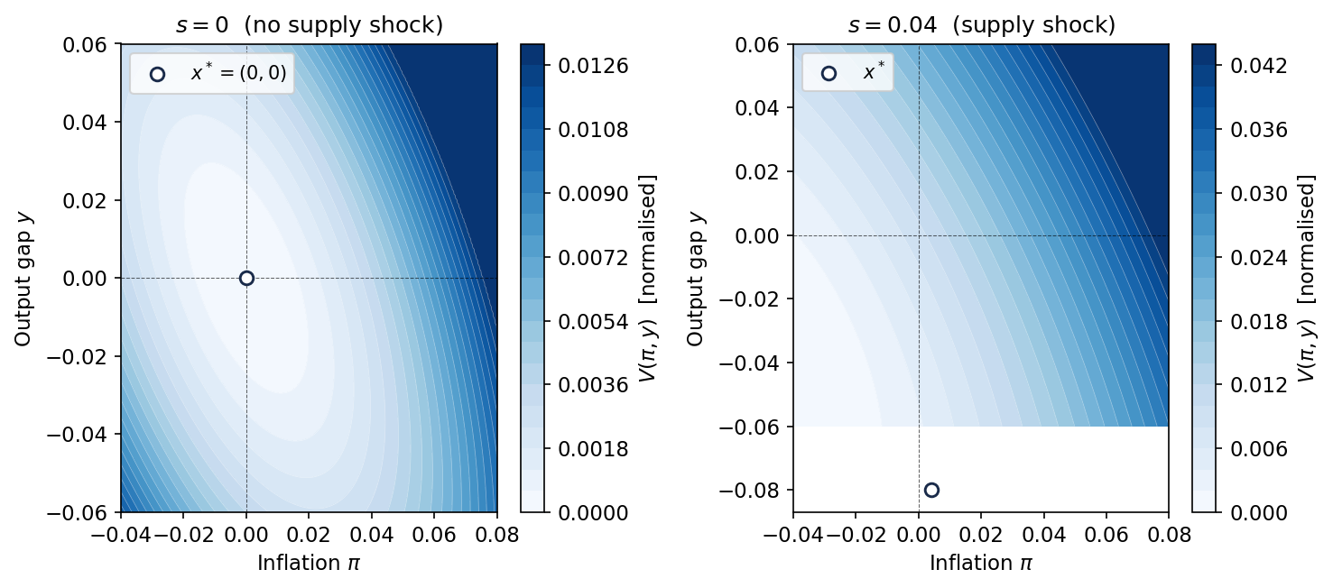
The Trap in Numbers

With the parameters above, numerical solution of the ARE gives the feedback gain $K$. The affine correction $p(s)$ is linear in $s$, so the feedforward premium and the displacement of $x^*$ both scale with the shock magnitude. For $s = 0.04$, the optimal equilibrium sits at strictly positive inflation and strictly negative output — the classic stagflation configuration.

**Figure 2.** **Optimal trajectories under and without a supply shock.** Each curve shows a path of the economy $(\pi_t, y_t)$ through time under the optimal policy, starting from a different initial condition. The arrows indicate the direction of travel. **Solid lines ($s = 0$):** every trajectory converges to the filled circle at the origin — zero inflation, zero output gap. The optimal policy successfully stabilises the economy regardless of where it starts. **Dashed lines ($s = 0.04$):** every trajectory still converges — the bank is still doing its job — but the destination has shifted. All paths lead to the lower circle: positive inflation, negative output. The bank cannot steer the economy to the origin while the supply shock persists. The distance between the two circles is the irreducible welfare cost of the shock.

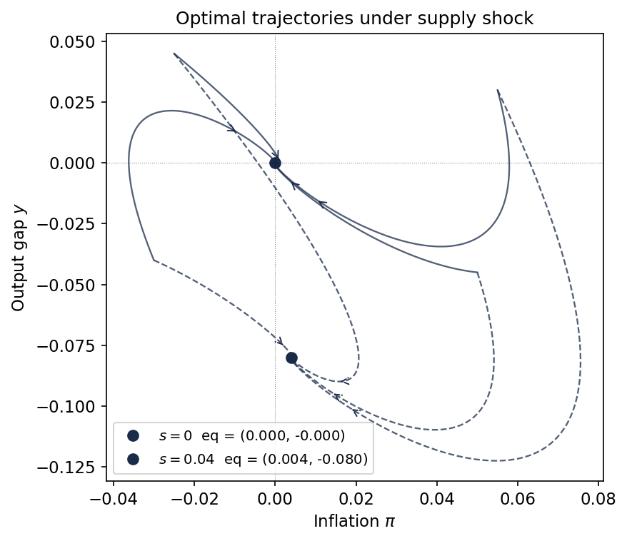
The phase portrait makes one thing plain: the bank is not failing. Both sets of trajectories converge; the optimal policy is working in both cases. The problem is that under a persistent supply shock, the best achievable outcome is not the ideal one.

Takeaway

The stagflation trap is not a puzzle about preferences, credibility, or central bank competence. It is a mathematical consequence of a linear economy driven by a persistent cost-push shock: the optimal policy cannot simultaneously zero inflation and the output gap. The HJB framework makes this exact — the shock enters through the affine correction $p(s)$, shifts the cost bowl, and displaces the optimal steady state in a way that no feedback rule can undo. The permanent welfare cost scales with $s^2$. Whether it can be reduced through alternative loss targets, commitment devices, or coordinated fiscal policy is the question that follows naturally from this model.

Interested in this line of work? Get in touch.