Two Worlds, One Price: Entropy and the Risk-Neutral Measure

Two Probabilities for One Asset

In classical physics, probability is a statement about a single world — a particle’s position has one distribution, determined by the Hamiltonian. Finance operates differently. Every option pricing model requires two probability measures: the **physical measure** $\mathbb{P}$, which describes how asset prices actually evolve, and the **risk-neutral measure** $\mathbb{Q}$, under which every discounted asset price is a martingale.

Under $\mathbb{P}$, equities earn a risk premium. Under $\mathbb{Q}$, they grow at the risk-free rate. One asset, two worlds. The question that connects thermodynamics to derivative pricing is: how different are these two worlds, and what does that difference cost?

The answer is relative entropy.

Relative Entropy — Distance Between Measures

The Kullback-Leibler divergence from $\mathbb{Q}$ to $\mathbb{P}$ is defined as

It measures how much information is gained — or how much surprise is introduced — when one replaces $\mathbb{P}$ with $\mathbb{Q}$. It is always non-negative, and equals zero if and only if the two measures are identical. It is not symmetric: $D_{KL}(\mathbb{Q}\|\mathbb{P}) \neq D_{KL}(\mathbb{P}\|\mathbb{Q})$ in general.

Physicists encountered this object long before information theorists named it. The **Gibbs free energy** of a distribution $\mathbb{Q}$ relative to a reference measure $\mathbb{P}$ is

where $U$ is potential energy, $T$ is temperature, and $H(\mathbb{Q}) = -\mathbb{E}^{\mathbb{Q}}[\log \mathbb{Q}]$ is the Gibbs entropy. Minimising $F$ over all $\mathbb{Q}$ subject to a fixed energy constraint produces the Boltzmann distribution $\mathbb{Q}^* \propto e^{-\beta U}$ — an exponential tilt of the reference measure. This minimisation is equivalent to minimising $D_{KL}(\mathbb{Q}\|\mathbb{P})$ subject to the same constraint.

The mathematical structure is identical in both fields: find the distribution closest to a reference, subject to a constraint.

From Girsanov to Gibbs

In continuous-time finance, the change of measure is governed by the **Girsanov theorem**. In a diffusion model with physical drift $\mu_t$ and volatility $\sigma_t$, the Radon-Nikodym derivative is

where $\lambda_t = (\mu_t – r)/\sigma_t$ is the **market price of risk** — the instantaneous Sharpe ratio of the risky asset. The measure $\mathbb{Q}$ is equivalent to $\mathbb{P}$ precisely when the Novikov condition $\mathbb{E}^{\mathbb{P}}[\exp(\frac{1}{2}\int_0^T \lambda_t^2 \, dt)] < \infty$ holds.

Substituting equation (3) into the definition (1) and simplifying:

The entropy cost of the risk-neutral measure is one-half the expected integrated squared Sharpe ratio. In a constant-parameter Black-Scholes model with $\lambda = (\mu – r)/\sigma$ constant, this reduces to

A market with no risk premium ($\mu = r$) has $\lambda = 0$ and $D_{KL} = 0$ — the two measures coincide and derivative prices equal their actuarial expectations under $\mathbb{P}$. The further the market departs from this benchmark, the higher the information cost of repricing under $\mathbb{Q}$.

The connection to Gibbs is now explicit. Equation (3) has the form $d\mathbb{Q}/d\mathbb{P} \propto \exp(-\theta \cdot X)$ — an exponential tilt of the reference measure, identical in structure to the Boltzmann factor $e^{-\beta U}$. The “energy” in the financial case is the stochastic integral $\int_0^T \lambda_t \, dW_t$. The “temperature” controls how far $\mathbb{Q}$ departs from $\mathbb{P}$. The Esscher transform used in actuarial science to price insurance risks has exactly the same form — this is not a coincidence.

Input:  mu (physical drift), r (risk-free rate), sigma (volatility), T (horizon)

1. Compute market price of risk:
      lambda = (mu - r) / sigma

2. Write the Radon-Nikodym derivative (Girsanov theorem):
      dQ/dP = exp( -lambda * W_T  -  (1/2) * lambda^2 * T )
   where W_T ~ N(0, T) under P.

3. Shift the Brownian motion to Q-world:
      W_T^Q = W_T + lambda * T       (W_T^Q is Brownian under Q)

4. Read off terminal densities in each world:
      log(S_T / S_0) ~ N( (mu - sigma^2/2)*T,  sigma^2*T )   under P
      log(S_T / S_0) ~ N( (r  - sigma^2/2)*T,  sigma^2*T )   under Q
   Same variance, different means — the densities are horizontal shifts of each other.

5. Compute entropy cost (equation 5):
      D_KL(Q || P) = (1/2) * lambda^2 * T

Output: lambda, D_KL, log-normal densities under P and Q

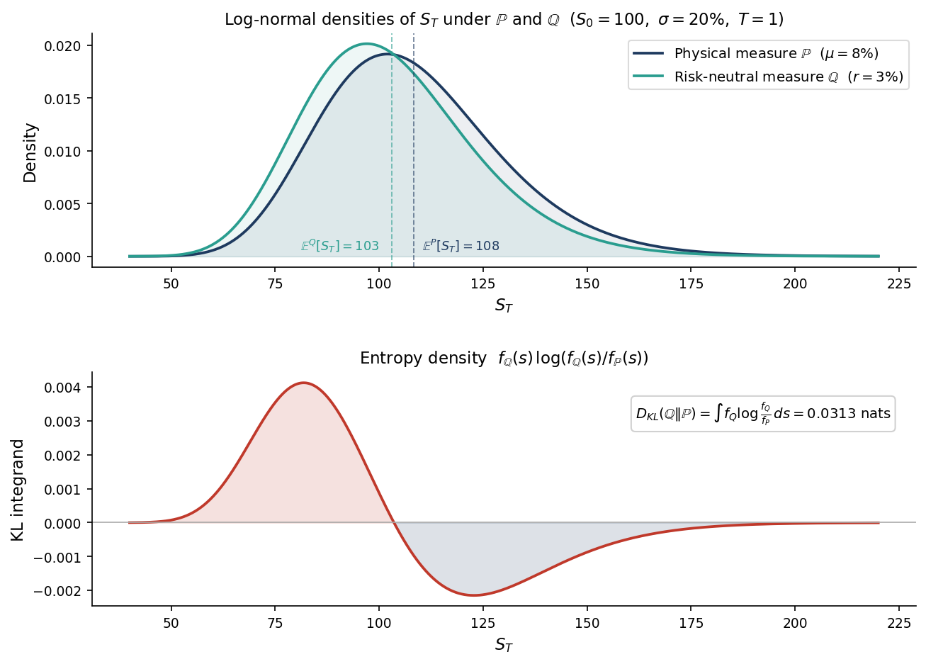
Figure 1 shows these two densities and the KL integrand $f_{\mathbb{Q}}(s)\log(f_{\mathbb{Q}}(s)/f_{\mathbb{P}}(s))$ whose integral equals $D_{KL}$. For $\lambda = 0.25$ and $T = 1$, the entropy cost is 0.0313 nats — small but non-zero, growing quadratically in $\lambda$ and linearly in horizon.

The lower panel goes negative in the right tail, and this is not an error. The KL integrand is negative wherever $f_{\mathbb{Q}}(s) < f_{\mathbb{P}}(s)$, that is, wherever $\mathbb{P}$ assigns more probability than $\mathbb{Q}$. Because $\mathbb{P}$ has a higher drift ($\mu = 8\%$ versus $r = 3\%$), it puts more weight on large values of $S_T$ — the right tail. In those regions, switching from $\mathbb{P}$ to $\mathbb{Q}$ actually reduces surprise: you are moving to a world that finds high prices less likely, so log$(f_\mathbb{Q}/f_\mathbb{P}) < 0$. The economic interpretation is direct: **under $\mathbb{Q}$, the upside that $\mathbb{P}$ considers realistic is systematically discounted**. Option sellers know this — they are being paid to price in a world that underweights the right tail relative to what history suggests. The positive region (low and mid prices, where $\mathbb{Q}$ has more mass than $\mathbb{P}$) dominates the negative region in the integral, and the total $D_{KL}$ is positive. The total entropy cost is the net information price of removing the risk premium.

The Minimal Entropy Martingale Measure

In the Black-Scholes model, $\mathbb{Q}$ is unique — the market is complete and $\lambda$ is pinned down by no-arbitrage. But in **incomplete markets** — models with jumps, stochastic volatility, or discrete trading — there are infinitely many measures equivalent to $\mathbb{P}$ under which discounted prices are martingales. No-arbitrage narrows the set but does not select a single element.

This is where entropy provides a canonical selection principle. The **minimal entropy martingale measure** (MEMM) is

where $\mathcal{M}$ is the set of all equivalent martingale measures. The MEMM selects the pricing measure that departs least from the physical dynamics — in the precise sense of relative information.

This is formally identical to the Gibbs variational principle: minimise free energy subject to a constraint. In physics, the constraint is a fixed energy expectation. In finance, it is the martingale condition $\mathbb{E}^{\mathbb{Q}}[e^{-rT} S_T] = S_0$. The solution in both cases has the exponential form in equation (3). For jump-diffusion models, the MEMM has been characterised explicitly by Frittelli (2000) and Fujiwara and Miyahara (2003). The resulting pricing measure damps the jump intensity in a way that minimises information loss relative to $\mathbb{P}$.

In stochastic volatility models (Heston, SABR), the MEMM imposes a specific relationship between the market prices of diffusion risk and volatility risk — one that can be tested against observed option surfaces.

What the Entropy Gap Tells You

Equation (4) has a direct empirical interpretation. The **variance risk premium** — the systematic gap between implied and realised volatility — is the entropy cost made observable.

If options are priced under a $\mathbb{Q}$ with $\lambda > 0$, implied variance $\sigma_{\mathbb{Q}}^2$ exceeds realised variance $\sigma_{\mathbb{P}}^2$ on average. The relationship is approximately

$$\sigma_{\mathbb{Q}}^2 – \sigma_{\mathbb{P}}^2 \approx \frac{2}{T} \cdot D_{KL}(\mathbb{Q} \| \mathbb{P})$$

This spread is observable in market data — it is the gap between VIX-squared and subsequent realised variance, one of the most robust and persistent anomalies in equity options markets. A large variance risk premium signals a large entropy gap: option sellers require compensation for operating in $\mathbb{Q}$-world rather than $\mathbb{P}$-world.

This framing also clarifies when Black-Scholes works well and when it breaks down. When the Sharpe ratio is small, $D_{KL}$ is small, the two measures are close, and pricing under $\mathbb{Q}$ is a minor perturbation of actuarial pricing. The formula degrades precisely as the entropy gap grows — in regimes with high risk premia, or in asset classes where jumps introduce a second source of risk that cannot be hedged.

Where This Shows Up in Practice

The entropy framework is not just a theoretical restatement of things already known. It has direct operational uses across quantitative finance.

**Variance risk premium harvesting.** The gap between implied variance (VIX-squared) and subsequent realised variance equals $\lambda^2$ — exactly twice the entropy cost per unit time. Systematic variance-selling strategies — short variance swaps, delta-hedged short straddles — are in effect harvesting this entropy gap. The entropy framing explains why the premium is persistent: it compensates for the information cost of operating under $\mathbb{Q}$ rather than $\mathbb{P}$.

**Entropy pooling.** Meucci (2008) introduced a portfolio construction technique in which an investor updates a prior distribution over returns to reflect views. The updated distribution is the one closest to the prior in KL sense subject to the views as equality constraints — formally identical to the MEMM problem. This is now standard practice at systematic asset managers and is implemented in most institutional risk systems.

**Robust portfolio optimisation.** Hansen and Sargent’s robust control framework models an investor who distrusts their reference measure $\mathbb{P}$. The investor optimises against the worst-case measure $\mathbb{Q}$ within a KL ball of radius $\delta$ around $\mathbb{P}$. The entropy radius $\delta$ is a direct, interpretable input: it parameterises how much model uncertainty the investor is willing to entertain. This framework is now used in central banking and macro policy research.

**Pricing in incomplete markets.** In jump-diffusion models (Kou, Merton), the risk-neutral measure is not unique. The MEMM gives the canonical pricing measure: it adjusts jump intensity and jump size distribution in the entropy-minimising direction. For exotic options — barriers, cliquets, variance swaps — the choice of $\mathbb{Q}$ can shift prices by 5–15%. The MEMM provides a principled, model-consistent default.

**Stress testing and scenario severity.** Regulatory stress scenarios (CCAR, FRTB) are implicitly alternative probability measures. The KL distance from the historical measure provides a natural severity metric — comparable across asset classes and scenarios, and consistent with the no-arbitrage structure of the model.

Takeaway

The change of measure at the heart of derivative pricing is not an accounting convention — it is an exponential tilt of the real-world probability measure, identical in structure to the Boltzmann distribution in statistical mechanics. The cost of that tilt is relative entropy: half the expected integrated squared Sharpe ratio. In complete markets this cost is uniquely fixed by no-arbitrage. In incomplete markets, minimising entropy provides a canonical and physically motivated selection principle. The variance risk premium — one of the most persistent empirical facts in options markets — is the directly observable signature of this entropy gap.

Interested in this line of work? Get in touch.