
Where the Force Vanishes Is Not Where It Rests
A Queue in Perfect Balance, Sitting Somewhere Else
Take one price level of a limit order book and watch the queue resting there. Orders join it and orders leave it, and both rates depend on how big the queue already is. A thin queue attracts the people who want to be near the front of it. A fat queue attracts the people who want to be filled at all, and it also attracts cancellations, because a fat queue is slow and the order behind it has been waiting.
Write $q$ for the size of the queue, $\lambda(q)$ for the rate at which orders arrive and $\theta(q)$ for the rate at which they leave without trading. The net force on the queue is the difference:
Somewhere there is a size at which the two exactly cancel. Call it $q^\ast$, the balance point: the queue size at which as much joins as leaves, the place where the force vanishes.
Now the question this post is about. Over a long morning, what is the average size of that queue?
The answer everyone reaches for is $q^\ast$. It is wrong, it is wrong by a computable amount, and the amount is not small. Below, three order books tuned to share exactly the same balance point rest 14.2% apart.
The Force Vanishes at the Balance Point. The Average Is Somewhere Else.
Give the queue its noise. The number of orders in it is a count, so the fluctuation scales with the square root of the count, which is the birth–death scaling every book model inherits:
Suppose this has settled down: $X_t$ is stationary, its law no longer moving. Then the average of $X_t$ is not moving either, and since the only thing pushing it is $b$, the average push has to be zero:
Read that carefully, because it is the whole post. The quantity that vanishes is $\mathbb{E}[b(X)]$ — the average of the force over every queue size the book visits. The balance point is defined by something else entirely: $b(q^\ast) = 0$, the force at one size. These are the same statement only if you may move the expectation inside $b$, and you may do that exactly when $b$ is a straight line.
That is Jensen’s inequality, in the place where it costs money. For a curved $b$,
so the resting average $\mathbb{E}[X]$ cannot be sitting at $q^\ast$. Expand $b$ about the mean $m = \mathbb{E}[X]$, keep two terms, and use $b(q^\ast)=0$ to trade $b(m)$ for the distance you are looking for:
Everything about the gap is in that fraction. The restoring strength $b^{\prime}(q^\ast)$ is negative — it has to be, or the queue would not be stable — so the sign of the gap is the sign of the curvature. A concave drift rests below its balance point; a convex one rests above it; a straight one rests exactly on it, and no amount of noise will move it. And the size of the gap is set by the variance: a noisier queue sits further from its balance point than a quiet one, with the same rates.
Three Books, One Balance Point, Three Different Homes
Fix an arrival floor $a_0 = 0.6$ and a noise $\sigma = 1$, and tune three rate pairs so that all three balance at exactly $q^\ast = 1.3$. Only the shape of the approach differs.
The concave book has sublinear arrivals and superlinear cancellations, $\beta = 0.30$ and $\gamma = 1.50$ — the shape the queue-reactive literature actually measures, going back to Huang, Lehalle and Rosenbaum’s fit to Paris futures. The linear book has $\beta = \gamma = 1$, the affine drift that every Ornstein–Uhlenbeck-flavoured model assumes. The convex book has sublinear cancellations, $\beta = 0.20$ and $\gamma = 0.75$.
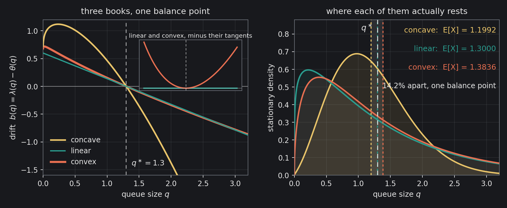
They do not rest in the same place, and they are not close. The concave book rests at $\mathbb{E}[X] = 1.1992$, which is 7.75% below its own balance point. The linear book rests at $1.3000$, on the balance point to twelve decimal places. The convex book rests at $1.3836$, 6.43% above. From end to end that is 14.2% of the balance point they all share, and every one of those books has arrivals and cancellations that cancel at precisely $1.3$.
The second-order formula calls the concave gap $-0.0922$ against a true $-0.1008$, and the convex gap $+0.1086$ against a true $+0.0836$. It gets the sign right always and the magnitude right to about a fifth, at a variance of $1.5$ against a mean of $1.3$ — which is to say, in a regime where “second order” is a generous description of the noise.
The most interesting curve in that figure is the one that looks like nothing. Look at the left panel: the convex drift is indistinguishable from the straight one. Its curvature is $b^{\prime\prime} = 0.0726$ against a restoring slope of $-0.5022$; you could not pick it out of a scatter plot of real arrivals with a year of data. It still moves the resting point by 6.43%.
The Gap Is Made of Noise
Since the correction is variance multiplied by curvature, turning the noise down should close it, and turning the noise up should open it in proportion to $\sigma^2$.
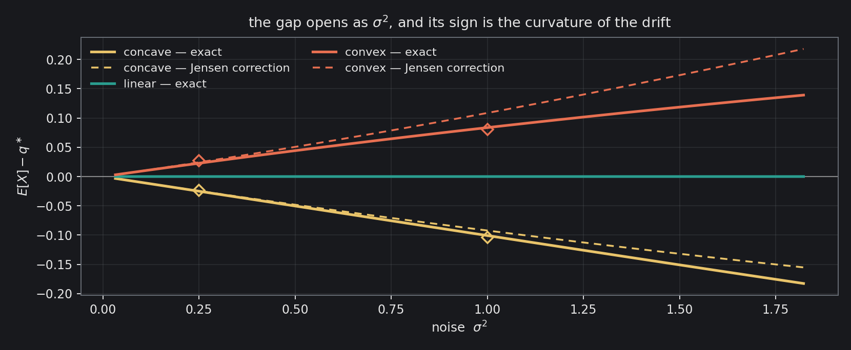
That teal line is the point of the figure. The affine book’s resting mean does not merely start at its balance point for small noise; it stays there, exactly, however violent the queue gets. Linearity is not an approximation that degrades. It is the one case where the intuition is a theorem, and it is the reason the intuition survives — every model anyone checks it against is linear.
The two curved books separate immediately and keep going, and the second-order correction tracks them until the variance stops being small and then, honestly, stops being enough. It over-predicts the convex gap by a half at the right-hand edge. It is the leading term of an expansion, not a closed form, and the figure is drawn out to where you can watch it fail rather than cropped to where it looks good.
Getting the Number
There is no need to simulate anything. A one-dimensional diffusion has its stationary density in closed form, and for this one the integral goes through by hand:
Two things live in that expression and both of them matter.
The exponent $2a_0/\sigma^2 – 1$ is the Feller exponent, and $a_0$ is the arrival rate at an empty queue. Set $a_0 = 0$ — let arrivals be purely size-reactive, which is the tempting simplification — and the origin becomes absorbing. The queue empties once and stays empty, there is no stationary law, and every number in this post evaporates. The floor is not a modelling nicety; it is the reason the question has an answer. When $2a_0 \geq \sigma^2$, as here, the queue never reaches zero at all.
The second thing is that when $\beta = \gamma = 1$ this collapses to a Gamma density, with shape $2a_0/\sigma^2$ and rate $2(c-a)/\sigma^2$, whose mean is $a_0/(c-a)$ — which is the balance point, algebraically, for every $\sigma$. That is the theorem of the previous section falling out of a formula that was never told about it.
Algorithm — The Resting Point of a State-Dependent Queue
input:  a0 > 0, a, beta, c, gamma, sigma          # rates and noise
        the arrival floor a0 must be strictly positive, or stop here:
        with a0 = 0 the origin absorbs and no stationary law exists

# ---- 1. the balance point: where the force vanishes ----------------------
b(q) <- a0 + a*q^beta - c*q^gamma
q*   <- the root of b, by bisection on any bracket [lo, hi] with b(lo)>0>b(hi)
        a bracket exists iff gamma > beta; otherwise cancellation never
        overtakes arrival and the queue is unstable

# ---- 2. the stationary density, in logs, on a log grid -------------------
u      <- linspace(log 1e-10, log 80, N)          # the grid is in log x
x      <- exp(u)
log w  <- (2*a0/sigma^2 - 1)*log x
          + (2/sigma^2) * ( a/beta * x^beta - c/gamma * x^gamma )
          + u                                     # the Jacobian: dx = x du
log w  <- log w - max(log w)                       # THEN exponentiate, never before
w      <- exp(log w)

# ---- 3. the resting point: where it actually sits ------------------------
Z    <- trapezoid(w, u)
m    <- trapezoid(x*w, u) / Z                      # E[X]
var  <- trapezoid(x*x*w, u) / Z  -  m*m
gap  <- m - q*                                     # the answer

# ---- 4. the correction, in closed form -----------------------------------
b1   <- b'(q*) ;  b2 <- b''(q*)                    # central differences are plenty
pred <- -0.5 * b2 * var / b1                       # sign from b2, size from var

# ---- 5. three things to check, none of them against each other -----------
CHECK 1  set beta = gamma = 1. The law is Gamma(2*a0/sigma^2, 2*(c-a)/sigma^2)
         and m must equal q* for EVERY sigma, in closed form.
CHECK 2  integrate b against the density: E[b(X)] must be 0 to machine
         precision, while b(m) must NOT be.
CHECK 3  integrate the SDE itself, full-truncation Euler, and compare the
         time-averaged mean. It shares no code with steps 2 to 4.

return q*, m, gap, pred

Two numerical traps, both of which returned a plausible wrong answer rather than
an error:
  - exponentiating before subtracting the maximum. The exponent passes several
    hundred before normalisation removes it, and the grid comes back as nan.
  - a UNIFORM grid in x. When 2*a0/sigma^2 < 1 the density has an integrable
    singularity at the origin and a uniform grid walks straight past it. The
    substitution x = exp(u) folds the singularity into the Jacobian.
What Is Checked, and Against What
Three checks, and the reason there are three is that a check sharing a code path with the thing it checks can only ever agree with it.
The first is the affine case, where the answer is known in closed form. The quadrature returns a mean of $1.300000$ and a variance of $1.408333$ against a Gamma law’s $1.300000$ and $1.408333$, and the gap from the balance point comes out at $1.1\times10^{-12}$ — zero, to the precision the arithmetic has. The second is the identity itself: integrating $b$ against each stationary density gives $\mathbb{E}[b(X)]$ of order $10^{-13}$ in all three books, while $b(\mathbb{E}[X])$ sits at $+0.1659$ for the concave one and $-0.0417$ for the convex one. The force at the average size is emphatically not zero; the average force is. The third is the differential equation itself, integrated by full-truncation Euler with five thousand paths, which reproduces the three means to $0.14\%$, $0.39\%$ and $0.21\%$ and touches no part of the density calculation.
The first of those checks earned its place immediately. The original quadrature ran on a uniform grid in $x$, and the affine book’s resting mean — which is $1.3$ for every noise level, in closed form, no approximation involved — drifted away from $1.3$ once $\sigma^2$ passed $1.2$. Nothing else showed it. Both curved books kept producing smooth, plausible, monotone curves the whole way out. The only thing that caught it was the one case with an answer to check against, and what it had caught was the density’s integrable singularity at the origin being quietly skipped by the grid. That is worth more than the theorem: a picture cannot tell you it is wrong, and neither can a residual computed on the same grid that is lying to you.
Why This Is Not a Curiosity
The concave book is not a case chosen to make a point. Sublinear arrivals and superlinear cancellations is what gets measured when anybody fits arrival and cancellation intensities against queue size on real order-by-order data. So the sign of the correction, for real books, is known in advance: a real queue rests below its balance point.
Which means the natural calibration is biased, and biased in one direction. Fit $\lambda$ and $\theta$ against queue size, solve $\lambda(q) = \theta(q)$, and quote the root as the typical depth at that level, and you have overstated the book. Here by 7.75%. And the error is proportional to the variance, so it is worst exactly where the queue is thin and jumpy and the reading matters most — and mildest where the queue is deep and placid and nobody needed the model anyway.
The same trap is set anywhere a nonlinear force is inverted for a resting state. Where does the inventory settle, given a nonlinear impact function. What spread does a market maker converge to, given a fill probability curved in the distance to the touch. What volatility does a feedback model relax to. In each case the equilibrium condition that is easy to solve is the force is zero here, and the quantity that is actually conserved is the average force is zero. They part company as soon as the force bends, and they part company by half the curvature times the variance, divided by the restoring strength.
What This Model Is Not
One price level, in isolation. Real levels are coupled — an order cancelled here often reappears one tick away, and the whole profile moves together when the price does. There is no price in this model at all, only a queue; depletion pricing, where the mid moves because a level emptied, is a different post and a longer one. The diffusion approximation replaces a counting process by a continuous one, which is safe for a hundred-lot queue and not safe for a five-lot queue, and five-lot queues are exactly where the small-cap book lives. The rates are constant in time, so nothing here knows about the open, the close, or a news print.
None of that touches the shape of the result, because the result does not depend on the model being right. It depends only on $b$ being curved and $X$ having variance. Where the force vanishes is not where the thing rests, and the distance between the two is not an error term. It is the curvature, paid for in noise.
Working on a pricing model or risk system? Let’s talk.