
Everybody Wants the Cheap Plug
A Mean Field Game: Ten Thousand Drivers, Two Cheap Plugs, One Hour
A fleet of vehicles is scattered across a city twenty kilometres wide and ten deep. All of them need charging, and they have an hour. Power is cheap in two places on the map — cheap in the west, slightly less cheap in the east — and expensive everywhere else.
Every driver pays for three things. The effort of getting somewhere, the price of power wherever they end up, and the queue they join when they arrive. The first two are fixed and knowable. The third is not: it is everybody else.
That last term is what makes this a game rather than an optimisation. Each driver’s best plan depends on what the crowd does, and what the crowd does is the sum of everybody’s best plan.
This is a mean field game, and it is about as simple as one gets. Two coupled partial differential equations, a cost that is quadratic in speed, and a single scalar that says how much a queue hurts. No common noise, no boundary, no heterogeneous agents, no major player — every one of those is a real extension and none of them is here. It is close to the first model you would write down if you had never written one before, and almost everything that makes the subject worth knowing is already in it.
The Mean Field Game System: One Equation Each, Pointing in Opposite Directions
Write $u(t,x)$ for the value function of one driver — the cost of the rest of their hour, if they are at $x$ at time $t$ and play optimally from there. Write $m(t,x)$ for the density of the whole fleet. The model is the pair:
The conditions that close them are $u(T,\cdot) = w_T V$ — wherever you end the hour you go on paying that price for a while — and $m(0,\cdot) = m_0$, the fleet where it starts.
The first line is Hamilton–Jacobi–Bellman. It runs backwards from the end of the hour, because you plan from where you want to end up. The second is Fokker–Planck. It runs forwards from now, because that is the direction crowds actually move in. The optimal move is
and a solution is a pair $(u,m)$ that agrees with itself: the plan that is optimal against the crowd, and the crowd that results from everyone playing that plan. That is a Nash equilibrium of a game with a continuum of players, and it is an $\varepsilon$-Nash equilibrium of the game with $N$ of them, with $\varepsilon = O(1/\sqrt{N})$.
Note what the coupling is not. There is no central router, no message passing, no driver who knows where any other driver is. Each one knows the statistical law of the crowd and best-responds to it. That is the whole of the mean field assumption.
The Trick That Makes It Solvable
Forward-backward systems are unpleasant. You cannot march in either direction, because each end needs the other. A naive attempt — discretise $\tfrac12|\nabla u|^2$ and iterate — diverged outright for us at every coupling strength worth drawing.
The quadratic Hamiltonian is the special case that gives way. Substituting $\varphi = e^{-u/\sigma^2}$ kills the nonlinear term exactly:
This is the Hopf–Cole transform, and the same one that turns Burgers’ equation into the heat equation. Setting $\psi = m/\varphi$, the density factorises as $m = \varphi\psi$ with $\psi$ solving the same linear equation forwards. So with the crowd $m$ held fixed, both halves of the system are linear parabolic problems that a Fourier split-step integrates exactly and unconditionally stably. The outer loop is then a damped Picard iteration on $m$ alone, walked up in $g$ from zero so that each solve warm-starts from the last.
Two things bit, and both are worth writing down.
The first: $\varphi$ and $\psi$ overflow double precision. Here $e^{V/\sigma^2}$ is around $10^{9}$ per unit time and it compounds over two hundred steps; the first version of the solver died inside `phi*psi` and returned `NaN`. They are carried normalised with their log-scale tracked alongside. Their product needs no scale at all, because it is renormalised and the mass really is one.
The second: the potential must be evaluated at the midpoint of each step. Taking it at $m[n]$ meant the backward sweep read the crowd at the right-hand end of its interval and the forward sweep at the left-hand end — first order, and inconsistent between the two halves of the same Strang step. It showed as a residual layer at the terminal time: $7.3\times 10^{-1}$ at the second-to-last step against $1.2\times10^{-1}$ anywhere in the interior, on a solution whose fixed point had converged to $9\times10^{-10}$. A converged iteration is not a correct one.
What the Fleet Chooses for Itself
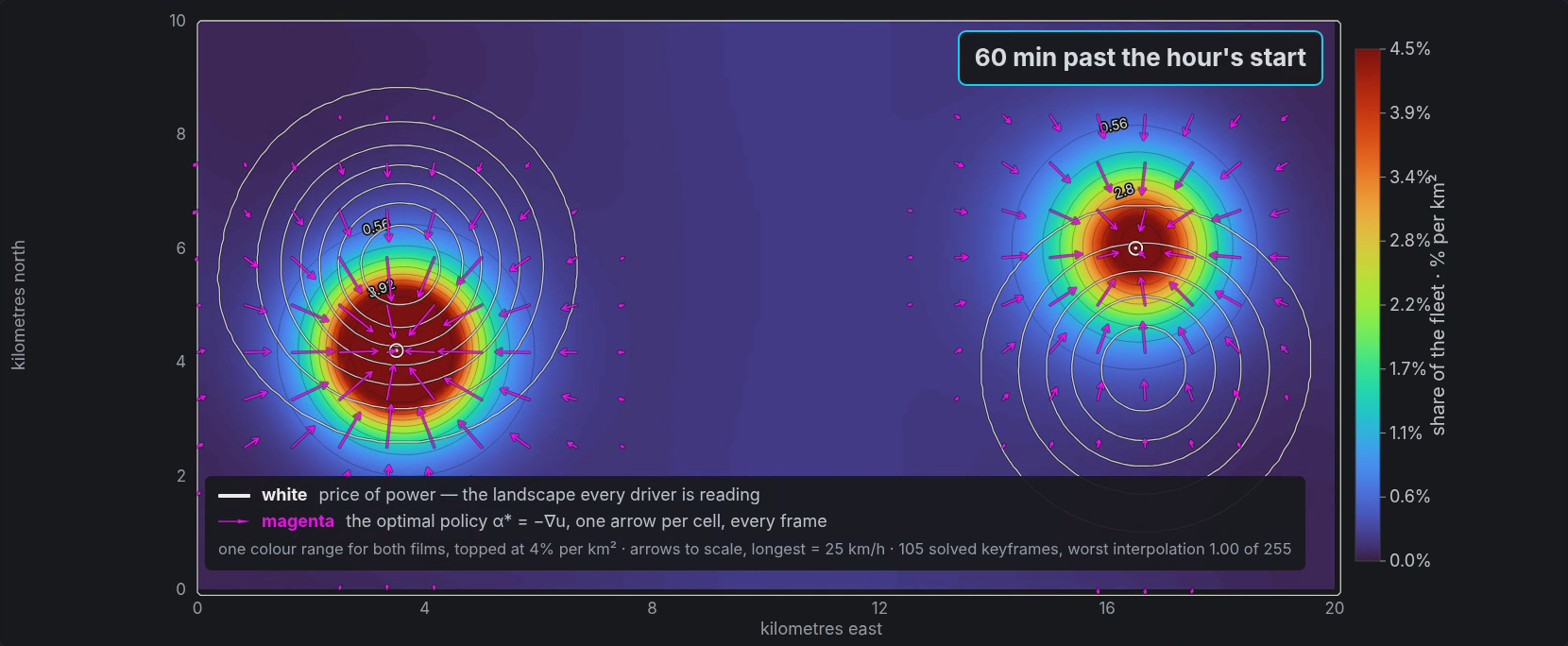
Colour is the fleet, as a share of it per square kilometre. The white rings are the price of power. The magenta arrows are $\alpha^* = -\nabla u$, one per cell, recomputed on every frame.
The first thing to notice is when the crowd decides. It does not pile into the cheap western basin, discover a queue and back out. At minute one, before anybody has gone anywhere, 44.3% of the fleet is already pointed east, away from the cheaper plug. In an equilibrium the queue is priced in before a single vehicle has moved. Drivers here do not learn about congestion; they anticipate it, because that is what “best response to the crowd’s law” means.
The second thing is where the drivers who leave actually go. With the queue term switched off entirely, 70.1% of the fleet ends the hour inside two kilometres of the western basin. Switch it on and that falls to 41.8% — but the eastern basin barely moves, from 24.6% to 25.4%. The congestion cost does not mostly redistribute the crowd between two plugs. It pushes it out of concentrations altogether, into the merely-adequate ground around them. The peak density falls from 30.1 to 10.0 per cent per square kilometre.
What the Same Fleet Would Choose Together
Now change exactly one thing. A driver joining a queue lengthens it for everyone already in it, and pays for none of that. A planner minimising the total bill sees the derivative of $g\!\int\! m^2$, which is $2gm$ — the marginal social cost, twice what the individual faces. Solve the identical system with the coupling doubled:
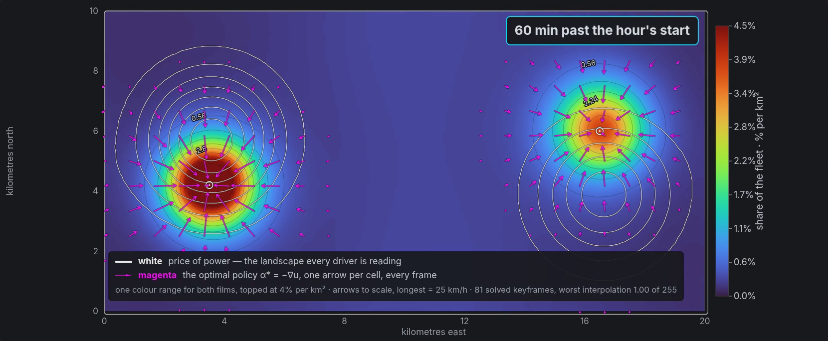
Same map, same fleet, same hour, same colour scale. Nobody is directed anywhere; every arrow is still that driver’s own best move against the crowd they face. But the busiest square kilometre now holds a third fewer vehicles — 6.8 per cent of the fleet against 10.0 — and the whole fleet pays less.
One Point Six Per Cent, And Nobody’s Fault
Scoring both flows with the same social cost functional:
gives 2.7367 for the fleet’s own equilibrium against 2.6936 for the planner’s. The ratio is the price of anarchy:
One point six per cent, wasted. It is a small number and the interesting part is who to blame for it, which is nobody. Every driver in this model solved their own problem exactly and played a best response to everybody else’s best response. Not one of them was irrational, careless or badly informed. The waste is not a mistake anyone made — it is a property of the equilibrium, and it does not go away by anybody trying harder.
That is also why exhortation does not work on problems shaped like this one. There is no message you can send to a driver who is already optimising.
The Fix Is a Number
What does work is a line Arthur Pigou wrote in 1920. Charge each driver the congestion they impose on everyone else:
levied at the place and the moment they are standing there. Add that to the individual’s running cost and their private problem becomes the planner’s problem: the selfish equilibrium is the coordinated one. You do not need to route anybody, ration anything, or know where a single vehicle is. You need one number, and you need it to vary with where the crowd actually is.
This is the practical content of the model, and it is why utilities and network operators care about mean field games rather than about simulating ten thousand vehicles. The object you need is $m$, not the vehicles.
The Algorithm
Algorithm — Mean Field Game by Hopf–Cole Split-Step
input:  price field V on the torus, start density m0, terminal weight wT,
        noise sigma, coupling g, grid NX x NY, Nt time steps, damping theta
dt <- T / Nt
uT <- wT * V                                  # where you end the hour still costs you
m  <- m0, copied to all Nt+1 time levels      # the crowd: the thing being solved for

repeat until max |m_new - m| < 1e-9:

    # ---- backwards: one driver's plan, given the crowd -------------------
    phi[Nt] <- exp(-uT / sigma^2)             # Hopf-Cole:  u = -sigma^2 * log(phi)
    for n = Nt down to 1:
        F <- V + g * (m[n] + m[n-1]) / 2      # the crowd at the interval's MIDPOINT
        phi[n-1] <- STEP(phi[n], F)
        divide phi[n-1] by its max, adding log(max) to a running scale
                                              # or it overflows double precision

    # ---- forwards: where the crowd goes, given that plan -----------------
    psi[0] <- m0 / phi[0]
    for n = 0 .. Nt-1:
        F <- V + g * (m[n] + m[n+1]) / 2      # the SAME potential the backward sweep saw
        psi[n+1] <- STEP(psi[n], F)
        rescale as above

    m_new <- phi * psi, normalised to unit mass at each time level
                                              # the scales are constant in space, so
                                              # normalising removes them exactly
    m <- (1 - theta) * m + theta * m_new       # damped: the undamped map diverges

u <- -sigma^2 * (log(phi) + running scale)    # undo Hopf-Cole, exactly
return m, u          and the optimal policy  alpha* = -grad u


STEP(f, F) is one Strang split-step of   df/dt = (sigma^2/2) * Laplacian(f) - (F/sigma^2) * f:
    f <- inverseFFT[ exp(-(dt/2) * (sigma^2/2) * k^2) * FFT[f] ]     # half a diffusion
    f <- f * exp(-dt * F / sigma^2)                                  # all of the potential
    f <- inverseFFT[ exp(-(dt/2) * (sigma^2/2) * k^2) * FFT[f] ]     # half a diffusion

Run the whole thing at g = 0 first, then at 0.3g, 0.6g, g, each starting from the last
answer. Cold-starting at the target coupling diverges outright.
What is checked, and against what
Four things, and not one of them against the scheme that produced the answer — a reference that shares the suspect code path can only ever agree with it.
The residuals are formed from the two equations at the top of this page using spectral derivatives, so $\varphi$ and $\psi$ appear nowhere in them. The HJB residual comes to $2.0\times10^{-2}$ against a term scale of $2.87$; Fokker–Planck to $1.0$ against $113.5$. Mass is conserved to $2\times10^{-16}$, and the density never goes negative. And the convergence order is measured rather than assumed: halve $\Delta t$ and the interior residuals fall by factors of 2.58 and 2.74 in $\log_2$, which is the second order the scheme is supposed to have.
One honest caveat about where the residual lives, because it is not uniform in time. It sits near $10^{-3}$ through the middle of the hour and then doubles at every step into the last few, mirrored at the first few. That is a start-up layer — the place where an exactly imposed terminal or initial condition meets a split-step propagation, and where a centred difference divides that first step’s error by $2\Delta t$. It is reported separately rather than averaged into a flattering maximum. A converged iteration is not a correct one, and the first version of this solver proved it: the fixed point had settled to $9\times10^{-10}$ while the potential was still being read at the wrong end of each interval.
What This Model Is Not
The map is a torus, which is a real simplification and a convenient one: it removes the boundary from the problem so that the interaction is the only thing on screen. Costs are quadratic in speed, which is what makes Hopf–Cole available and is otherwise an assumption. Congestion enters linearly in $m$, so the marginal social cost is exactly twice the private one — pick a different congestion law and the factor changes, though the Pigouvian argument does not. There is no queue with a service rate, no state of charge, no vehicle that gives up and goes home, and no price that responds to demand.
What survives all of that is the shape of the answer, and it is the part worth carrying: a crowd of individually flawless optimisers lands somewhere worse than it needs to, the gap is computable, and the instrument that closes it is a price that tracks the crowd rather than a rule that overrides it.
Where the Pictures Come From
Both panels are frames of the film above, which is drawn by `d3-contour` from the solved fields — the same bytes, not a redrawing of them. Each exhibit finishes its hour a few seconds before its beat ends and then holds the solved state still, so the frame to take is one from the middle of that pause — the same moment of the modelled hour in both, whatever their different lengths on screen.
There is no matplotlib anywhere in this piece. One drawing engine made the film, the two figures above and the thumbnail.
The solver, the script that lifted these frames, and the figures themselves are archived beside this post’s own markdown, so everything above can be re-derived rather than taken on trust.
Working on a pricing model or risk system? Let’s talk.