When Sampling Faster Makes You Wrong

Two Names for the Same Volatility

An econometrician handed a day of tick data has a natural estimate of how much the price moved: add up the squared returns. A probabilist handed a stochastic differential equation has a natural object measuring the same thing: the quadratic variation of the process. These are not two ideas — they are one idea seen from two eras. The discrete estimator is the sample version of the continuous quantity, and as the sampling grid refines, the first converges to the second.

That convergence is the theoretical bridge between financial econometrics and continuous-time modelling, and it comes with a clean, almost irresistible prescription: to measure volatility better, sample faster. Real market data punishes that instinct. Past a certain frequency, sampling faster makes the estimate worse — without bound. This post shows exactly where the bridge holds, where it collapses, and how a two-scale estimator rebuilds it.

Realized Variance Estimates a Quadratic Variation

Model the efficient log-price as a driftless Itô process whose volatility can vary through the day:

$$dX_t = \sigma_t\,dW_t, \qquad [X]_T = \int_0^T \sigma_t^2\,dt \;\equiv\; IV.$$

$(1)$

The object $[X]_T$ is the quadratic variation — the integrated variance $IV$, the total quantity of randomness the path accumulated over $[0,T]$. Its discrete estimator, formed from returns on a grid $t_0 < t_1 < \dots < t_n = T$, is the realized variance, and the foundational result of high-frequency econometrics is that it is consistent for exactly this integral:

$$RV_n = \sum_{i=1}^{n}\big(X_{t_i}-X_{t_{i-1}}\big)^2 \;\xrightarrow[n\to\infty]{}\; [X]_T = \int_0^T \sigma_t^2\,dt.$$

$(2)$

Take the limit seriously and the advice writes itself: more increments, more information, less error. Nothing in equation (2) argues for stopping.

The Trap: What You Actually Observe Is Not the Price

The catch is that no one observes $X$. Trades print at the bid or the ask, in discrete ticks, with a lag — a whole market microstructure sits between the efficient price and the number on the tape. Model that gap as additive noise:

$$Y_{t_i} = X_{t_i} + U_{t_i},\quad U \sim \mathrm{iid}(0,\sigma_U^2),\qquad \mathbb{E}\big[RV_n^{Y}\big] = \underbrace{\int_0^T \sigma_t^2\,dt}_{\text{signal, fixed}} \;+\; \underbrace{2\,n\,\sigma_U^2}_{\text{noise, grows}}.$$

$(3)$

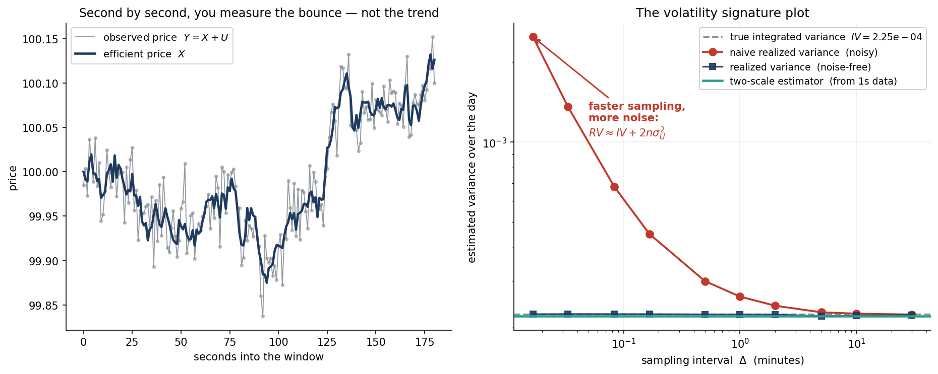
Read the two terms. The signal is the integral you want — it does not care how finely you sample. The noise term is $2n\sigma_U^2$, and it is proportional to the number of increments $n$. Every time you halve the sampling interval you double $n$, and the bias doubles with it. As $\Delta \to 0$ the estimator does not converge to $IV$; it diverges to infinity. The left panel of the figure shows why in miniature: over a three-minute window the efficient price (navy) drifts a little, but each one-second observation (grey) jumps around it by more than the drift itself. Differencing the grey series at one-second spacing measures the bounce, not the move.

Recovering the Truth from Noisy Data: Two Scales

The fix, due to Zhang, Mykland, and Aït-Sahalia, is to use two sampling scales and let them cancel the noise. Compute the realized variance on all the data — this is dominated by the noise term $2n\sigma_U^2$ — and also average the realized variance over $K$ interleaved sparse subgrids, which sees far less noise. A weighted difference annihilates the bias and leaves a consistent estimate of the integrated variance:

$$\widehat{[X]}_T^{\,\text{TSRV}} = \frac{1}{\,1-\bar n/n\,}\left(\overline{RV}^{(K)} – \frac{\bar n}{n}\,RV_n^{Y}\right),\qquad \bar n = \frac{n-K+1}{K}.$$

$(4)$

The slow scale carries the signal; the fast scale measures the noise so it can be subtracted. Crucially, this is computed from the same one-second data that made the naive estimator explode — nothing is thrown away.

Algorithm — Two-Scale Realized Variance

input: noisy log-prices Y_0 .. Y_n over the day, subgrid count K
# fast scale: RV on every increment (noise-dominated)
RV_all <- sum over i=1..n of (Y_i - Y_{i-1})^2
# slow scale: average RV over the K interleaved sparse subgrids
RV_avg <- (1 / K) * sum over i=K..n of (Y_i - Y_{i-K})^2
n_bar  <- (n - K + 1) / K
# subtract the fast-scale noise estimate, then debias
TSRV   <- (RV_avg - (n_bar / n) * RV_all) / (1 - n_bar / n)
return TSRV

The Experiment

Simulate a trading day of one-second efficient prices under a U-shaped intraday volatility, add microstructure noise, and compute the realized variance at sampling intervals from one second to thirty minutes — with and without noise — alongside the two-scale estimator built from the full one-second series. Average over many days to trace the volatility signature plot.

Python 3.13 — The Volatility Signature Plot and the Two-Scale Estimator

import numpy as np
import matplotlib
matplotlib.use("Agg")
import matplotlib.pyplot as plt

# Efficient log-price  dX = sigma(t) dW  on one trading day t in [0,1]
# (6.5h = 23400 one-second bars). Observed price Y = X + U carries i.i.d.
# microstructure noise U ~ N(0, a^2). Realized variance estimates the
# quadratic variation  IV = int_0^1 sigma(t)^2 dt.
Nfine = 23400
dtf = 1.0 / Nfine
tg = np.linspace(0.0, 1.0, Nfine + 1)
shape = 0.7 + 0.9 * np.cos(2 * np.pi * tg) ** 2               # U-shaped intraday vol
sig = 0.5 * (shape[:-1] + shape[1:])
sig *= np.sqrt((0.015 ** 2) / np.mean(sig ** 2))             # daily vol 1.5%
IV = np.sum(sig ** 2 * dtf)
a = 2.2e-4                                                    # noise std ~2.2 bps

def day(rng):
    X = np.concatenate([[0.0], np.cumsum(sig * rng.normal(0.0, np.sqrt(dtf), Nfine))])
    return X, X + rng.normal(0.0, a, Nfine + 1)

def tsrv(Y, K=100):                                          # two-scale (ZMA 2005)
    n = len(Y) - 1
    rv_avg = np.sum((Y[K:] - Y[:-K]) ** 2) / K
    rv_all = np.sum(np.diff(Y) ** 2)
    nbar = (n - K + 1) / K
    return (rv_avg - (nbar / n) * rv_all) / (1 - nbar / n)

ms = np.array([1, 2, 5, 10, 30, 60, 120, 300, 600, 1800])   # sample every m seconds
dmin = ms / 60.0                                            # minutes per sample
rng = np.random.default_rng(0)
M = 300
rv_naive = np.zeros(len(ms)); rv_clean = np.zeros(len(ms)); ts = 0.0
for _ in range(M):
    X, Y = day(rng)
    ts += tsrv(Y)
    for j, m in enumerate(ms):
        idx = np.arange(0, Nfine + 1, m)
        rv_naive[j] += np.sum(np.diff(Y[idx]) ** 2)
        rv_clean[j] += np.sum(np.diff(X[idx]) ** 2)
rv_naive /= M; rv_clean /= M; ts /= M

NAVY, TEAL, RED, GREY = "#1e3a5f", "#2a9d8f", "#c0392b", "#8a8f98"
fig, (axL, axR) = plt.subplots(1, 2, figsize=(12.6, 5.2), facecolor="white",
                               gridspec_kw={"width_ratios": [1, 1.08]})

# LEFT: 3-minute zoom, efficient trend vs noisy observed price
Xz, Yz = day(np.random.default_rng(4))
w = 180
sec = np.arange(w + 1)
P = 100.0 * np.exp(Xz[:w + 1]); Pobs = 100.0 * np.exp(Yz[:w + 1])
axL.plot(sec, Pobs, color=GREY, lw=0.9, alpha=0.9, zorder=1, label="observed price  $Y = X + U$")
axL.plot(sec, Pobs, "o", color=GREY, ms=2.6, alpha=0.55, zorder=2)
axL.plot(sec, P, color=NAVY, lw=2.2, zorder=3, label="efficient price  $X$")
axL.set_xlabel("seconds into the window"); axL.set_ylabel("price")
axL.set_title("Second by second, you measure the bounce — not the trend", fontsize=11.3)
axL.legend(loc="upper left", framealpha=0.85, fontsize=9.5)
axL.spines[["top", "right"]].set_visible(False)

# RIGHT: the volatility signature plot
axR.axhline(IV, color=GREY, lw=1.6, ls="--", label=f"true integrated variance  $IV = {IV:.2e}$")
axR.plot(dmin, rv_naive, "o-", color=RED, lw=1.8, ms=7, label="naive realized variance  (noisy)")
axR.plot(dmin, rv_clean, "s-", color=NAVY, lw=1.6, ms=6, alpha=0.9, label="realized variance  (noise-free)")
axR.axhline(ts, color=TEAL, lw=2.2, label="two-scale estimator  (from 1s data)")
axR.annotate("faster sampling,\nmore noise:\n$RV\\approx IV + 2n\\sigma_U^2$",
             xy=(dmin[0], rv_naive[0]), xytext=(0.05, 1.05e-3),
             color=RED, fontsize=10, fontweight="bold", ha="left",
             arrowprops=dict(arrowstyle="->", color=RED, lw=1.4))
axR.set_xscale("log"); axR.set_yscale("log")
axR.set_xlabel("sampling interval  $\\Delta$  (minutes)")
axR.set_ylabel("estimated variance over the day")
axR.set_title("The volatility signature plot", fontsize=12)
axR.legend(loc="upper right", framealpha=0.9, fontsize=9)
axR.grid(True, which="major", alpha=0.22)
axR.spines[["top", "right"]].set_visible(False)

fig.tight_layout(pad=1.4)
fig.savefig("fig_1.png", dpi=150, bbox_inches="tight")

**Figure 1.** Left: a three-minute window of one trading day. The efficient price $X$ (navy) drifts smoothly, while each one-second observation $Y = X + U$ (grey) bounces around it by more than the drift itself — differencing the grey series measures the noise, not the move. Right: the volatility signature plot. Naive realized variance under microstructure noise (red) diverges as the sampling interval $\Delta \to 0$, reaching more than ten times the true integrated variance at one-second sampling; the noise-free realized variance (navy) is unbiased at every frequency, and the two-scale estimator (teal), computed from the same one-second data, lands on the true $IV$ (grey dashed).

What the Plot Says

The two red data points on the left are the whole story. At one-second sampling the naive estimator reports a variance eleven times too large — a “volatility” of roughly 5% for a day whose true figure is 1.5%. Slow the sampling to five or ten minutes and the red curve settles onto the truth, which is precisely the folklore rule that practitioners reached for years before the theory caught up: sample every five minutes and no faster. The signature plot explains that rule as a bias–variance compromise, not a law — coarse enough that the $2n\sigma_U^2$ term is negligible, fine enough that sampling error stays small.

The noise-free curve (navy) makes the diagnosis exact. It is flat on the true integrated variance at every frequency, because equation (2) has no bias term — the entire pathology in the red curve is the noise, nothing else. And the two-scale estimator (teal) shows the compromise is unnecessary: fed the raw one-second series that sent the naive estimator to eleven times the truth, it returns the integrated variance to within a couple of percent. You do not have to throw away 299 out of every 300 observations to escape the noise; you have to model it.

The Econometric Moral

The realized-variance–quadratic-variation bridge is real, and it is the reason a continuous-time SDE is the right object behind a stream of discrete prices. But consistency is a statement about a model, and the model observed here was $X$, not $Y$. The moment you take the noise seriously — as an econometrician staring at a signature plot must — the naive limit theorem inverts, and the optimal amount of data is emphatically not “all of it.” Modern high-frequency econometrics is, in large part, the project of writing down estimators whose limit theory survives contact with $Y$: two-scale and multi-scale estimators, realized kernels, pre-averaging. Each is a different way of doing what the teal line does here — reaching through the microstructure to touch the quadratic variation of the SDE underneath.

Working on a pricing model or risk system? Let’s talk.