The Neuron as an Ornstein–Uhlenbeck Process

A Leaky Bucket That Remembers Its Rest

A neuron’s membrane behaves like a leaky capacitor. Synaptic currents charge it up; through the membrane’s own conductance it steadily leaks back toward a resting voltage. Written as a differential equation, the subthreshold voltage $V(t)$ of the standard leaky integrate-and-fire neuron obeys

$$\tau\,\partial_t V = -(V – V_{\mathrm{rest}}) + R\,I(t),$$

$(1)$

where $\tau$ is the membrane time constant and $R\,I(t)$ is the input. A cortical neuron receives thousands of tiny, roughly independent synaptic events per second. By the central limit theorem their sum is well approximated by a mean drive plus Gaussian white noise, $R\,I(t) = \mu + \sigma\sqrt{\tau}\,\xi(t)$. Substitute that in and the membrane equation becomes a stochastic differential equation:

$$\mathrm{d}V = \tfrac{1}{\tau}\,(\mu – V)\,\mathrm{d}t + \sigma\,\mathrm{d}W_t.$$

$(2)$

This is the Ornstein–Uhlenbeck process — the same mean-reverting diffusion a quant reaches for when modelling a stationary spread. The dictionary is exact: the membrane leak is the mean reversion (rate $\tfrac{1}{\tau}$), the effective input $\mu$ is the long-run mean, and the synaptic bombardment is the diffusion $\sigma$. A neuron, below threshold, is running an OU process.

But a Neuron Has a Threshold

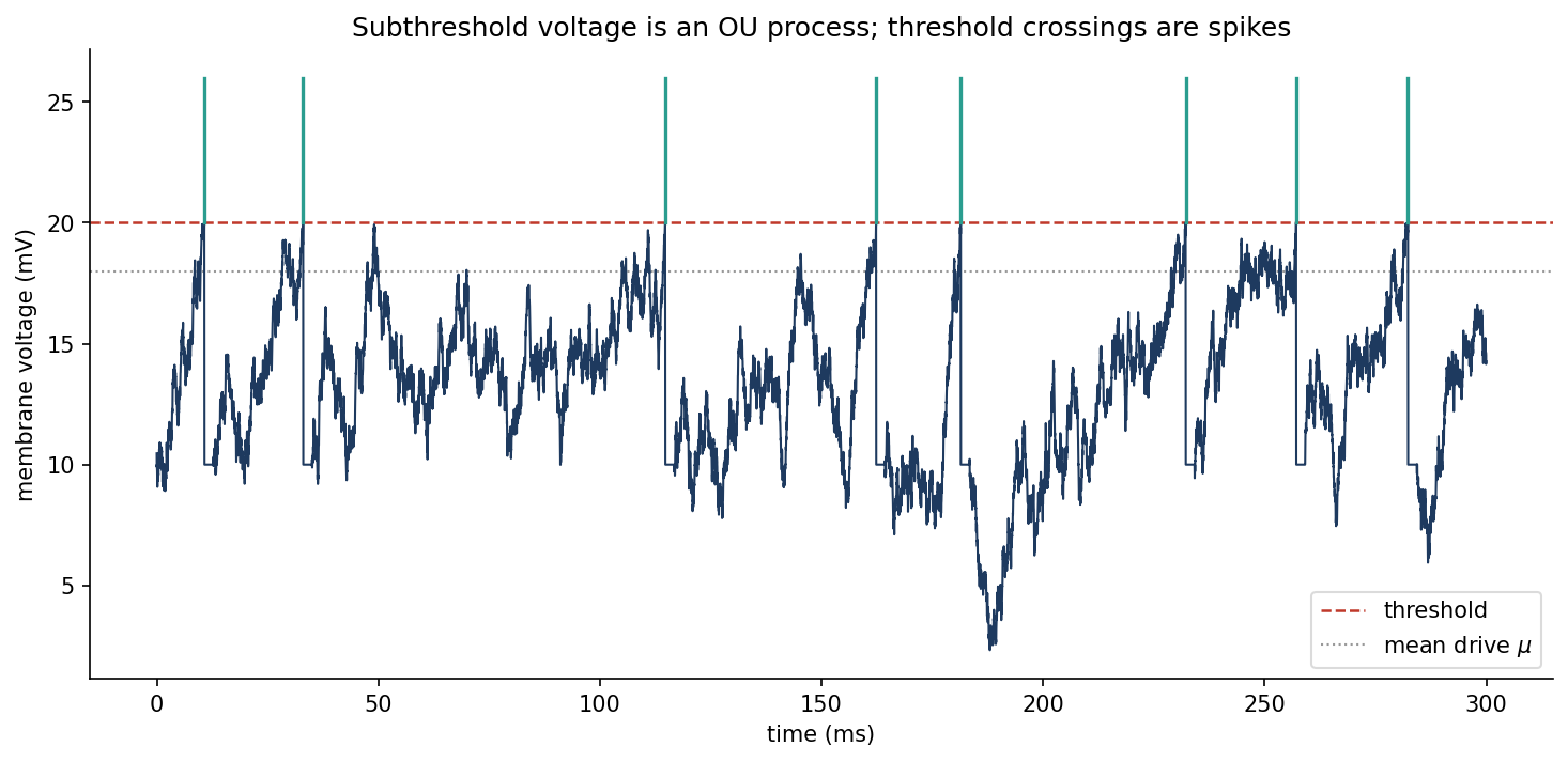
The analogy would be a curiosity if it stopped at the subthreshold voltage. It does not. When $V$ reaches a spike threshold $V_{\mathrm{th}}$, the neuron fires an action potential and the voltage is reset to $V_{\mathrm{reset}}$, after which it integrates again. So the neuron is not merely an OU process — it is an OU process with an absorbing boundary at $V_{\mathrm{th}}$ and an instantaneous reset. Simulate it and the structure is plain: a mean-reverting wander that occasionally touches the line and starts over.

Python 3.13 — The OU Neuron: Voltage Trace and the f–I Curve from First Passage

import numpy as np
import matplotlib
matplotlib.use("Agg")
import matplotlib.pyplot as plt
from scipy.special import erfcx
from scipy.integrate import quad

NAVY, TEAL, RED = "#1e3a5f", "#2a9d8f", "#c0392b"

# leaky integrate-and-fire / OU parameters (mV, ms)
tau, Vth, Vre, tref, sigV = 20.0, 20.0, 10.0, 2.0, 5.0
s_in = sigV * np.sqrt(2.0 / tau)        # white-noise amplitude for stationary std = sigV

def simulate(mu, T, dt=0.02, seed=0):
    rng = np.random.default_rng(seed)
    n = int(T / dt); V = np.empty(n); v = Vre; ref = 0; spikes = []
    sq = s_in * np.sqrt(dt)
    for i in range(n):
        if ref > 0:
            ref -= 1; V[i] = Vre; continue
        v += (mu - v) / tau * dt + sq * rng.standard_normal()
        if v >= Vth:
            spikes.append(i * dt); V[i] = Vth
            v = Vre; ref = int(tref / dt)            # spike + reset + refractory
        else:
            V[i] = v
    return np.arange(n) * dt, V, np.array(spikes)

def rate_theory(mu):                                  # Ricciardi/Siegert first-passage rate (Hz)
    d = sigV * np.sqrt(2.0)
    integ, _ = quad(lambda u: erfcx(-u), (Vre - mu) / d, (Vth - mu) / d, limit=200)
    return 1000.0 / (tref + tau * np.sqrt(np.pi) * integ)

def rate_noiseless(mu):                               # deterministic LIF: silent, then periodic
    return 0.0 if mu <= Vth else 1000.0 / (tref + tau * np.log((mu - Vre) / (mu - Vth)))

# Figure 1 — voltage trace with spikes
t, V, sp = simulate(mu=18.0, T=300.0, seed=3)
fig, ax = plt.subplots(figsize=(10, 5), facecolor="white")
ax.axhline(Vth, color=RED, lw=1.2, ls="--", label="threshold")
ax.axhline(18.0, color="#999999", lw=1.0, ls=":", label=r"mean drive $\mu$")
ax.plot(t, V, color=NAVY, lw=1.0)
for x in sp:
    ax.plot([x, x], [Vth, Vth + 6], color=TEAL, lw=1.6)
ax.set_xlabel("time (ms)"); ax.set_ylabel("membrane voltage (mV)")
ax.set_title("Subthreshold voltage is an OU process; threshold crossings are spikes")
ax.legend(framealpha=0.7, loc="lower right"); ax.spines[["top", "right"]].set_visible(False)
fig.tight_layout(pad=1.5); fig.savefig("fig_1.png", dpi=150, bbox_inches="tight"); plt.close(fig)

# Figure 2 — f-I curve: noiseless vs OU first passage, validated by Monte Carlo
mus = np.linspace(10.0, 30.0, 41)
r_th = np.array([rate_theory(m) for m in mus])
r_nl = np.array([rate_noiseless(m) for m in mus])
mus_mc = np.linspace(11.0, 29.0, 10)
r_mc = np.array([len(simulate(m, T=40000.0, seed=1)[2]) / 40000.0 * 1000.0 for m in mus_mc])
fig, ax = plt.subplots(figsize=(10, 5), facecolor="white")
ax.plot(mus, r_nl, color="#999999", lw=1.6, ls="--", label="noiseless (hard threshold)")
ax.plot(mus, r_th, color=NAVY, lw=2.0, label="OU first-passage (Ricciardi)")
ax.plot(mus_mc, r_mc, "o", color=RED, ms=6, label="Monte Carlo")
ax.axvline(Vth, color=RED, lw=1.0, ls=":", alpha=0.7)
ax.set_xlabel(r"mean input drive  $\mu$  (mV)"); ax.set_ylabel("firing rate (Hz)")
ax.set_title("Noise smooths the transfer function: the f-I curve from OU first passage")
ax.legend(framealpha=0.7); ax.spines[["top", "right"]].set_visible(False)
fig.tight_layout(pad=1.5); fig.savefig("fig_2.png", dpi=150, bbox_inches="tight"); plt.close(fig)

**Figure 1.** A single simulated neuron. The membrane voltage (navy) mean-reverts toward the drive $\mu = 18$ mV, buffeted by synaptic noise; each time it reaches the threshold (red) it emits a spike (teal) and resets to $V_{\mathrm{reset}} = 10$ mV. The subthreshold path is a textbook Ornstein–Uhlenbeck trajectory.

The Firing Rate Is a First-Passage Time

Here is where the quantitative reader should sit up. The interval between two spikes is the time the OU process takes to travel from $V_{\mathrm{reset}}$ up to $V_{\mathrm{th}}$ for the first time — a first-passage time, the very object used to price barrier options and model default. The neuron’s firing rate is simply the reciprocal of the mean interval (plus a refractory dead time $t_{\mathrm{ref}}$):

$$r = \Big(t_{\mathrm{ref}} + \mathbb{E}\big[\,T_{V_{\mathrm{reset}}\to V_{\mathrm{th}}}\,\big]\Big)^{-1}.$$

$(3)$

The mean first-passage time of an OU process across a fixed barrier is not a simulation artefact to be measured — it has a closed form, derived by Siegert in 1951 and standard in computational neuroscience (the Ricciardi integral). With $\sigma_V = \sigma\sqrt{\tau/2}$ the stationary standard deviation of the free membrane voltage,

$$\frac{1}{r} = t_{\mathrm{ref}} + \tau\sqrt{\pi}\int_{(V_{\mathrm{reset}}-\mu)/\sqrt{2}\,\sigma_V}^{(V_{\mathrm{th}}-\mu)/\sqrt{2}\,\sigma_V} e^{u^2}\big(1 + \operatorname{erf} u\big)\,\mathrm{d}u.$$

$(4)$

The integrand grows explosively, but the substitution $e^{u^2}(1+\operatorname{erf} u) = \operatorname{erfcx}(-u)$ — the scaled complementary error function — makes it numerically painless. This is the neuron’s transfer function: input drive in, firing rate out.

Noise Dissolves the Threshold

What does that transfer function look like, and why should we care? Compare two neurons. The noiseless one is a brutal switch: for any mean drive below $V_{\mathrm{th}}$ it is silent forever, and the instant the drive exceeds threshold it fires with a clockwork rate. Its f–I curve is a wall — flat zero, then a sudden rise.

Now add the synaptic noise back. The wall dissolves.

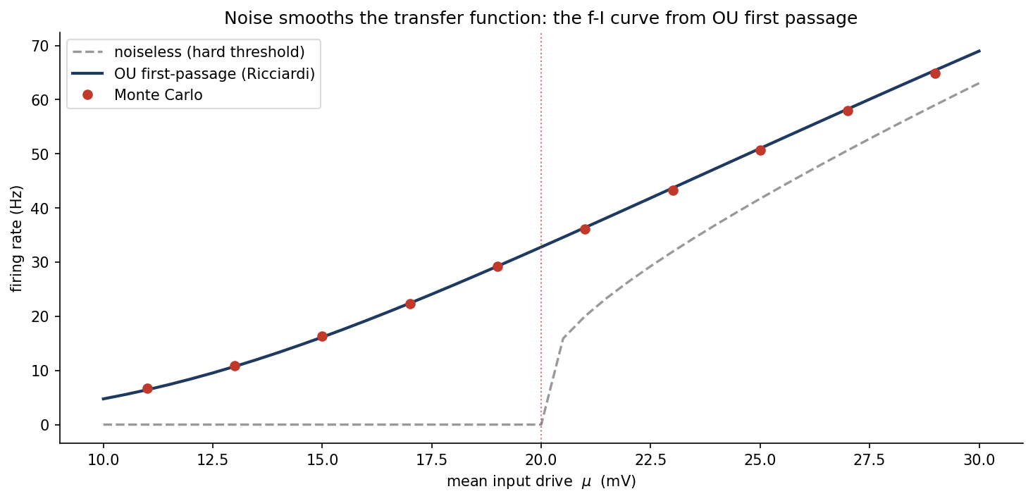
**Figure 2.** Firing rate versus mean drive. The noiseless neuron (grey dashed) is silent below threshold and abruptly periodic above it. The OU neuron (navy, from the Ricciardi first-passage formula) fires *below* threshold — random fluctuations carry it over — and its response is a smooth, graded curve. Monte-Carlo simulation (red) confirms the formula to better than 1 Hz.

Two things change, and both matter. First, the neuron fires even when the average input is below threshold: fluctuations occasionally push the voltage over the line, so the drive no longer has to clear the barrier on its own. Second, and more importantly, the transfer function becomes smooth and graded rather than all-or-none. Noise converts a binary switch into an analog device with a continuous input–output relationship — the property a network needs to compute with rates rather than mere presence or absence of spikes. In the computational-neuroscience literature this is why fluctuation-driven regimes are studied at all: the noise is not a defect to be filtered away, it is what makes graded neural computation possible.

Same Mathematics, a Different Universe

The point of the exercise is not that a neuron happens to resemble a financial spread. It is that a single object — the Ornstein–Uhlenbeck process with an absorbing barrier — and a single question — when does it first cross? — appear in two fields that never cite each other. The barrier-crossing integral that gives a neuron its firing rate is structurally the same computation that gives a down-and-out option its price or a firm its default probability. Learn the first-passage machinery once and it pays out across every domain where something mean-reverts until it hits a line. The neuron is just an unusually beautiful place to find it.

Interested in applying these ideas to your work? Get in touch.