The Neuron as a Density: Fokker–Planck with a Reset

One Path, or the Whole Cloud

In the previous post a cortical neuron turned out to be an Ornstein–Uhlenbeck process with an absorbing barrier: the membrane voltage $V$ mean-reverts toward its input drive, synaptic noise buffets it, and each time it touches the spike threshold $V_{\mathrm{th}}$ it fires and is reset to $V_{\mathrm{reset}}$. The firing rate came out of a first-passage time — how long, on average, does the path take to travel from reset to threshold — and the closed form for that mean crossing time gave the neuron’s transfer function.

That is the backward view: fix a starting voltage, ask a question about the future of one trajectory. There is a second, complementary view, and it is the one a physicist or a PDE person reaches for. Forget the single path. Take a large population of these neurons — or one neuron watched for a long time, it comes to the same thing — and ask how the density of membrane voltages evolves. That question is answered by the forward equation, and it is where the neuron stops being a curiosity and starts being a network.

The Boundary Condition That Makes It a Neuron

The Fokker–Planck equation for the density $p(V,t)$ of an OU process is standard: drift transports the density, diffusion spreads it. What makes this one a neuron is not the equation, it is the boundary condition.

$$\partial_t p = \partial_V\!\left[\frac{V-\mu}{\tau}\,p\right] + \frac{s^2}{2}\,\partial_V^2 p \; + \; r(t-t_{\mathrm{ref}})\,\delta\!\left(V – V_{\mathrm{reset}}\right).$$

$(1)$

Read the two extra pieces carefully, because between them they contain the entire biology.

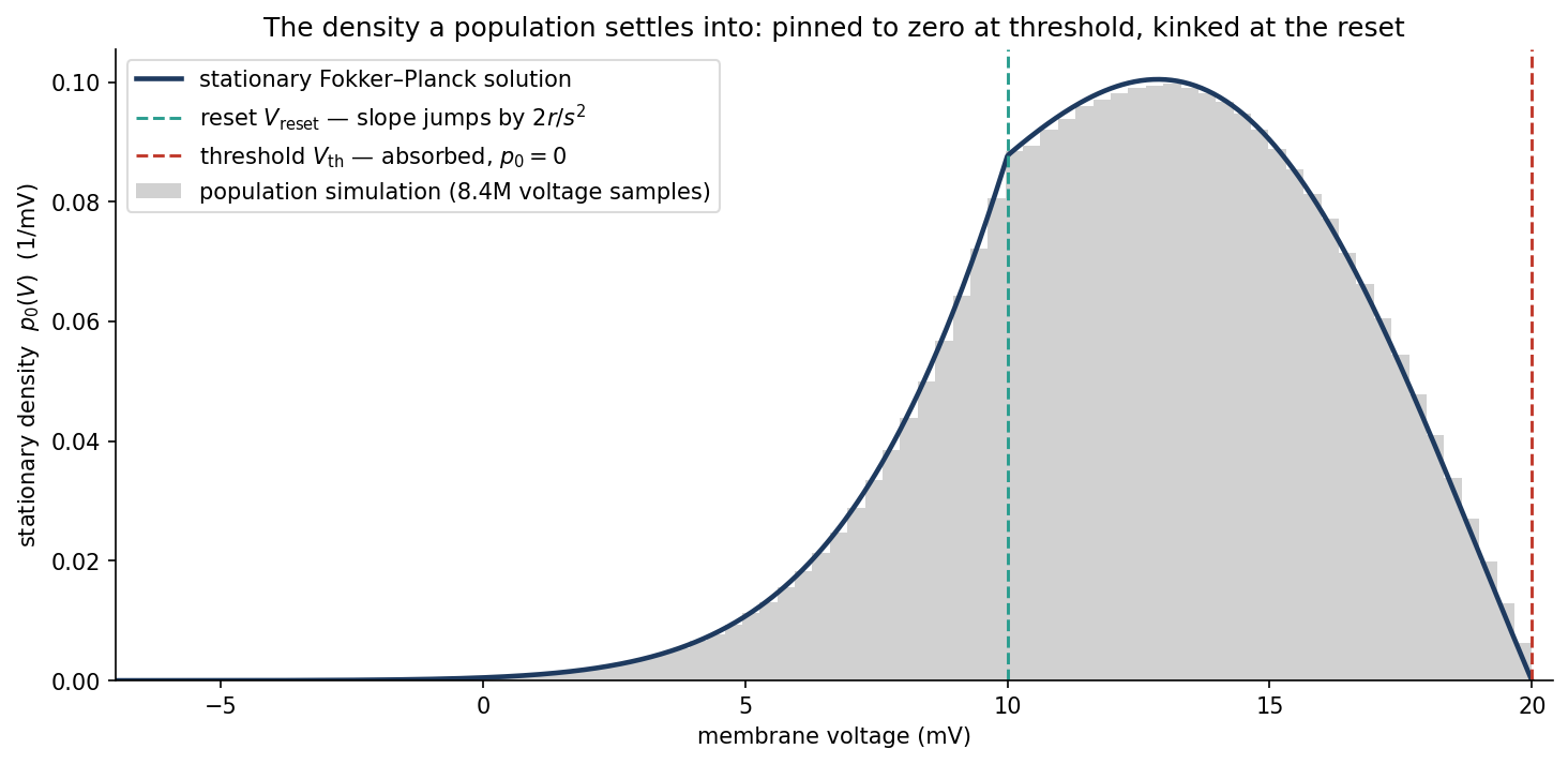
First, the threshold absorbs. Any probability that reaches $V_{\mathrm{th}}$ leaves the subthreshold world — the neuron has spiked. So the density is pinned to zero there, and the rate at which probability drains out through that boundary is the firing rate. It is a probability flux, and the flux of a diffusion at an absorbing wall is the gradient of the density:

$$p(V_{\mathrm{th}},t) = 0, \qquad r(t) \;=\; -\,\frac{s^2}{2}\,\partial_V p(V,t)\Big|_{V=V_{\mathrm{th}}}.$$

$(2)$

The firing rate is a slope. Not an average of anything, not a statistic to be estimated — the steepness with which the population density approaches the threshold it is forbidden to occupy.

Second, that escaped probability does not vanish from the universe. After a refractory dead time $t_{\mathrm{ref}}$ the neuron reappears at the reset voltage, which is the delta source in Equation 1: whatever leaves at $V_{\mathrm{th}}$ is reinjected at $V_{\mathrm{reset}}$. The system is conservative, but in a circular way — it is a diffusion on a line whose exit is wired back into its middle. That single feature is what separates this PDE from every textbook Fokker–Planck equation, and it leaves a visible mark: the reinjected flux forces the derivative of the density to jump discontinuously at the reset, by exactly $2r/s^2$. The stationary density is continuous but kinked, and the size of the kink is the firing rate.

Python 3.13 — Stationary Fokker–Planck Density, the Rate as a Flux, and the Network Fixed Point

import numpy as np
import matplotlib
matplotlib.use("Agg")
import matplotlib.pyplot as plt
from scipy.special import erfcx
from scipy.integrate import quad
from scipy.optimize import brentq

NAVY, TEAL, RED, GREY = "#1e3a5f", "#2a9d8f", "#c0392b", "#999999"

# the same neuron as the previous post (units: mV, ms)
tau, Vth, Vre, tref, sigV = 20.0, 20.0, 10.0, 2.0, 5.0
s2 = 2.0 * sigV**2 / tau        # diffusion coeff of dV = (mu - V)/tau dt + s dW


def rate_backward(mu):
    """Ricciardi/Siegert mean-first-passage rate (Hz) — the BACKWARD equation's answer."""
    d = sigV * np.sqrt(2.0)
    integ, _ = quad(lambda u: erfcx(-u), (Vre - mu) / d, (Vth - mu) / d, limit=200)
    return 1000.0 / (tref + tau * np.sqrt(np.pi) * integ)


def shape(V, mu):
    """Stationary FP density divided by the rate, p_0(V)/r  (units: ms/mV).
       p_0(V) = (2r/s^2) e^{-(V-mu)^2/2sigV^2} * int_{max(V,Vre)}^{Vth} e^{(u-mu)^2/2sigV^2} du."""
    z = lambda x: (x - mu) / (np.sqrt(2.0) * sigV)
    b = z(Vth)
    out = np.empty_like(np.atleast_1d(V), dtype=float)
    for i, v in enumerate(np.atleast_1d(V)):
        a = z(max(v, Vre))
        # factor e^{b^2} pulled out of the integral so the integrand never overflows
        I, _ = quad(lambda u: np.exp(u * u - b * b), a, b, limit=200)
        out[i] = (2.0 / s2) * np.exp(-((v - mu) ** 2) / (2.0 * sigV**2)) \
                 * np.sqrt(2.0) * sigV * np.exp(b * b) * I
    return out


def v_arr(V):
    return np.array([V])


def rate_forward(mu):
    """Rate fixed by normalising the FORWARD equation's stationary density:
       r * int p_0/r dV + r*tref = 1."""
    mass, _ = quad(lambda V: shape(v_arr(V), mu)[0], mu - 12 * sigV, Vth, limit=400)
    return 1000.0 / (mass + tref)          # mass carries units of ms


def simulate_population(mu, N=4000, T=1500.0, dt=0.02, burn=400.0, seed=7):
    """Vectorised LIF population. Returns subthreshold voltage samples + the MC rate (Hz)."""
    rng = np.random.default_rng(seed)
    v = Vre + sigV * rng.standard_normal(N)
    ref = np.zeros(N, dtype=int)
    sq = np.sqrt(s2 * dt)
    samples, spikes, neuron_ms = [], 0, 0.0
    for i in range(int(T / dt)):
        act = ref == 0
        v[act] += (mu - v[act]) / tau * dt + sq * rng.standard_normal(int(act.sum()))
        fired = act & (v >= Vth)
        v[fired] = Vre
        ref[fired] = int(tref / dt)
        ref[ref > 0] -= 1
        if i * dt > burn:
            spikes += int(fired.sum())
            neuron_ms += N * dt
            if i % 25 == 0:
                samples.append(v[ref == 0].copy())
    return np.concatenate(samples), spikes / neuron_ms * 1000.0


MU = 18.0
r_fwd, r_bwd = rate_forward(MU), rate_backward(MU)
volts, r_mc = simulate_population(MU)
active_frac = 1.0 - r_fwd * tref / 1000.0        # mass of p_0: the non-refractory fraction

# Figure 1 — the stationary density, closed form vs population
Vg = np.linspace(MU - 5 * sigV, Vth, 700)
p0 = shape(Vg, MU) * r_fwd / 1000.0              # true p_0(V), integrates to active_frac

fig, ax = plt.subplots(figsize=(10, 5), facecolor="white")
h, edges = np.histogram(volts, bins=100,
                        weights=np.full(volts.size, active_frac / volts.size))
ax.bar(edges[:-1], h / np.diff(edges), width=np.diff(edges), align="edge",
       color=GREY, alpha=0.45, linewidth=0,
       label=f"population simulation ({volts.size/1e6:.1f}M voltage samples)")
ax.plot(Vg, p0, color=NAVY, lw=2.2, label="stationary Fokker–Planck solution")
ax.axvline(Vre, color=TEAL, lw=1.4, ls="--", label=r"reset $V_{\mathrm{reset}}$ — slope jumps by $2r/s^2$")
ax.axvline(Vth, color=RED, lw=1.4, ls="--", label=r"threshold $V_{\mathrm{th}}$ — absorbed, $p_0=0$")
ax.set_xlim(Vg[0], Vth + 0.4)
ax.set_ylim(0, None)
ax.set_xlabel("membrane voltage (mV)")
ax.set_ylabel(r"stationary density  $p_0(V)$  (1/mV)")
ax.set_title("The density a population settles into: pinned to zero at threshold, kinked at the reset")
ax.legend(framealpha=0.7, loc="upper left")
ax.spines[["top", "right"]].set_visible(False)
fig.tight_layout(pad=1.5)
fig.savefig("fig_1.png", dpi=150, bbox_inches="tight")
plt.close(fig)

# Figure 2 — the network sets its own rate:  r = Phi(mu_ext - g r)
g, MU_EXT = 0.55, 30.0                            # recurrent inhibition (mV per Hz), external drive
r_star = brentq(lambda r: rate_forward(MU_EXT - g * r) - r, 0.0, 200.0, xtol=1e-8)
mu_star = MU_EXT - g * r_star

mus = np.linspace(6.0, 30.0, 55)
phi = np.array([rate_forward(m) for m in mus])

w_damp = 0.35                                     # undamped Picard oscillates: |g * dPhi/dmu| > 1
r_it, traj_d, traj_u = 0.0, [0.0], [0.0]
for _ in range(12):
    r_it = (1 - w_damp) * r_it + w_damp * rate_forward(MU_EXT - g * r_it)
    traj_d.append(r_it)
r_u = 0.0
for _ in range(12):
    r_u = rate_forward(MU_EXT - g * r_u)
    traj_u.append(r_u)

fig, axes = plt.subplots(1, 2, figsize=(12, 5), facecolor="white")
ax = axes[0]
ax.plot(mus, phi, color=NAVY, lw=2.2, label=r"single-neuron transfer function  $\Phi(\mu)$")
ax.plot(mus, (MU_EXT - mus) / g, color=TEAL, lw=2.0, ls="--",
        label=r"recurrent constraint  $\mu = \mu_{\mathrm{ext}} - g\,r$")
ax.plot([mu_star], [r_star], "o", color=RED, ms=9, zorder=5,
        label=f"operating point ({mu_star:.1f} mV, {r_star:.1f} Hz)")
ax.set_xlim(mus[0], mus[-1])
ax.set_ylim(0, float(phi.max()) * 1.05)
ax.set_xlabel(r"mean drive  $\mu$  (mV)")
ax.set_ylabel("firing rate (Hz)")
ax.set_title("Two constraints, one intersection")
ax.legend(framealpha=0.7, loc="upper left")
ax.spines[["top", "right"]].set_visible(False)

ax = axes[1]
ax.plot(range(len(traj_u)), traj_u, "-o", color=GREY, lw=1.5, ms=4,
        label="undamped: oscillates")
ax.plot(range(len(traj_d)), traj_d, "-o", color=NAVY, lw=1.8, ms=5,
        label=f"damped ($w={w_damp}$): converges")
ax.axhline(r_star, color=RED, lw=1.2, ls="--", label=f"fixed point  {r_star:.2f} Hz")
ax.set_xlabel("iteration $n$")
ax.set_ylabel("firing rate (Hz)")
ax.set_title("Finding it: the loop gain is larger than one")
ax.legend(framealpha=0.7, loc="upper right")
ax.spines[["top", "right"]].set_visible(False)

fig.tight_layout(pad=1.5)
fig.savefig("fig_2.png", dpi=150, bbox_inches="tight")
plt.close(fig)

print(f"forward  (FP normalisation)  r = {r_fwd:.5f} Hz")
print(f"backward (Ricciardi MFPT)    r = {r_bwd:.5f} Hz   |diff| = {abs(r_fwd - r_bwd):.2e}")
print(f"Monte Carlo population       r = {r_mc:.5f} Hz")
print(f"network: mu* = {mu_star:.2f} mV, r* = {r_star:.2f} Hz")

**Figure 1.** The stationary density of membrane voltages at a drive of $\mu = 18$ mV. The closed-form Fokker–Planck solution (navy) sits on top of a histogram of 8.4 million voltage samples from a simulated population of 4,000 neurons (grey). Three features are structural, not accidental: the density vanishes at the threshold (red) because the boundary absorbs; its slope jumps discontinuously at the reset (teal) because escaped probability is reinjected there; and the sharpness of the approach to threshold is, quite literally, the firing rate.

Forward and Backward Must Agree

Stationarity turns the PDE into an ordinary differential equation, and it is one you can integrate by hand. Between the reset and the threshold the flux is constant and equal to $r$; below the reset it is zero. Solving with the integrating factor and imposing $p_0(V_{\mathrm{th}}) = 0$ gives the density up to one unknown constant:

$$p_0(V) \;=\; \frac{2r}{s^2}\;e^{-(V-\mu)^2/2\sigma_V^2}\int_{\max(V,\,V_{\mathrm{reset}})}^{V_{\mathrm{th}}} e^{(u-\mu)^2/2\sigma_V^2}\,\mathrm{d}u .$$

$(3)$

The unknown constant is the firing rate itself, and there is exactly one thing left to impose — that the neurons all have to be somewhere. Either a neuron is sitting at some subthreshold voltage, or it is in its refractory period, and the probabilities must sum to one:

$$\int_{-\infty}^{V_{\mathrm{th}}} p_0(V)\,\mathrm{d}V \; + \; r\,t_{\mathrm{ref}} \;=\; 1 .$$

$(4)$

That single normalisation condition determines $r$. Nothing else is needed. And here is the check that matters: the rate you get this way — from the forward equation, by demanding that a density integrate to one — is the same number as the mean-first-passage rate from the previous post, which came from the backward equation and a question about a single trajectory. Run the code and the two agree to ten decimal places (25.77295 Hz at $\mu = 18$ mV, differing by $4 \times 10^{-10}$ Hz). They must: they are the same operator, adjoint to each other, answering the same physical question from opposite ends. Seeing the two computations meet is the cheapest available proof that neither is wrong.

The Monte-Carlo population comes in at 25.16 Hz — about 2% low, and not from randomness. An Euler–Maruyama step checks the threshold only at grid points, so it silently misses excursions that cross and come back within a step. The bias is systematic, it shrinks with the step size, and it is exactly the pathology that makes the discretisation of a barrier its own subject.

The Network Chooses Its Own Firing Rate

Now the payoff, and the reason the forward view was worth the trouble. So far the drive $\mu$ was ours to set. In a real cortical circuit it is not: a neuron’s input is the output of thousands of other neurons in the same population, most of them inhibitory. Raise the population’s firing rate and you raise the inhibition every neuron receives, which lowers the drive. Write that feedback in its simplest honest form, $\mu = \mu_{\mathrm{ext}} – g\,r$, and the network’s operating point is no longer something we impose. It is a fixed point:

$$r_\star \;=\; \Phi\!\left(\mu_{\mathrm{ext}} – g\,r_\star\right),$$

$(5)$

where $\Phi$ is the transfer function we just built out of the Fokker–Planck solution. The neuron’s rate depends on its input; its input depends on the population’s rate; the population’s rate is its own. The circuit has to solve for itself.

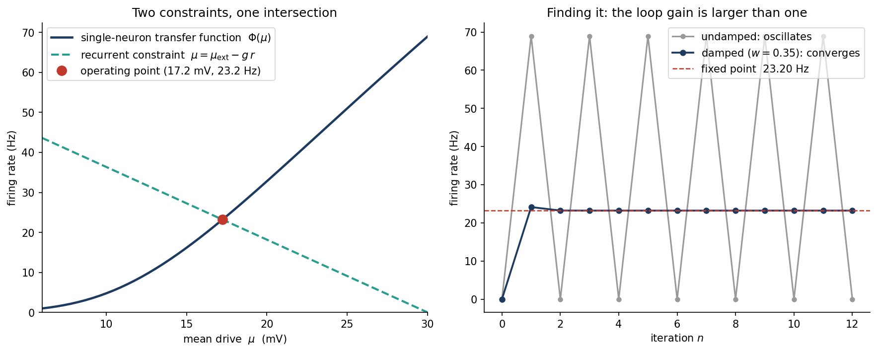
**Figure 2.** Left: the self-consistent operating point of a recurrent, inhibition-dominated population. The single-neuron transfer function $\Phi(\mu)$ (navy) and the recurrent constraint $\mu = \mu_{\mathrm{ext}} – g\,r$ (teal) are two curves in the same plane, and the network lives where they cross — at 23.2 Hz, against the 69 Hz the same external drive would produce with the feedback cut. Right: finding that point. Naive iteration overshoots and oscillates forever, because the loop gain $|g\,\Phi’|$ exceeds one; damping the update by $w = 0.35$ lands it in three steps.

Two things in that figure are worth more than the neuroscience. The first is that the intersection is the answer — feedback converts a transfer function into a self-consistency problem, and the solution belongs to the circuit, not to any neuron in it. The second is what happens when you go looking for it: the obvious iteration, plug in a rate and get a rate back, diverges. It flips between 0 and 69 Hz forever, because the slope of the response times the strength of the feedback is bigger than one. Damp the update and it converges immediately. Anyone who has solved a mean-field model, a general-equilibrium fixed point, or a coupled Fokker–Planck system has met that same wall and reached for the same underrelaxation.

The Structure Is the Point

Strip the biology away and what remains is a diffusion on an interval, absorbed at one end, reinjected in the middle, whose exit flux is fed back into its own drift until the whole thing is self-consistent. That description does not mention neurons, and it does not need to. It is the same machinery that prices a barrier option with a rebate, that closes a heterogeneous-agent economy where each agent’s policy depends on a distribution that their own behaviour generates, and that defines a mean-field game.

The neuron did not teach us the mathematics. It gave us an unusually vivid place to watch the mathematics work — a boundary you can point at, a flux you can measure in hertz, and a fixed point that a piece of cortex has to find several thousand times a second.

Need a reliable numerical implementation for your problem? Get in touch.