Cholesky vs Eigendecomposition: Two Ways to Sample Correlated Gaussians

One Problem, Two Factorizations

Almost every Monte Carlo engine in finance needs the same primitive: draw a vector of jointly normal variables with a prescribed covariance. Correlated asset returns, correlated risk factors, correlated shocks in a scenario generator — all of it reduces to sampling $X \sim \mathcal{N}(0, \Sigma)$ for a given covariance (or correlation) matrix $\Sigma$.

The recipe is standard. Find any matrix $A$ that “square-roots” the covariance, draw independent standard normals $Z$, and mix them:

$$X = A Z, \qquad A A^\top = \Sigma, \qquad Z \sim \mathcal{N}(0, I_n).$$

$(1)$

This works because the covariance of $A Z$ is $A\,\mathrm{Cov}(Z)\,A^\top = A A^\top = \Sigma$, exactly what we wanted. Any $A$ with $A A^\top = \Sigma$ does the job — and that freedom is the whole story, because there are two popular choices of $A$ and they behave very differently.

The Cholesky Route

The Cholesky factorization writes $\Sigma$ as a lower-triangular matrix times its transpose:

$$\Sigma = L L^\top, \qquad X = L Z.$$

$(2)$

It is the natural default: it costs about $n^3/3$ floating-point operations, it is numerically clean, and the triangular structure makes the subsequent multiply cheap. If you take one thing away, it is this — when $\Sigma$ is genuinely positive definite, Cholesky is the right answer.

The catch is in that condition. Cholesky exists only for a positive definite matrix. Hand it a matrix with a single non-positive eigenvalue and it does not approximate, warn, or degrade — it raises an error and stops.

The Eigendecomposition Route

The spectral route diagonalizes $\Sigma$ into its eigenvectors $Q$ and eigenvalues $\Lambda$, then takes the symmetric square root:

$$\Sigma = Q \Lambda Q^\top, \qquad A = Q \Lambda^{1/2}, \qquad X = Q \Lambda^{1/2} Z.$$

$(3)$

This is the same construction that underlies principal component analysis, and it is strictly more work than Cholesky — a full symmetric eigensolve carries a noticeably larger constant. What you buy for that cost is information: the decomposition hands you the eigenvalues explicitly. When one of them is negative, you can see it, and you can fix it.

The Cost of Each

When $\Sigma$ is well-behaved, the only question is speed — and inside a Monte Carlo loop that factorizes repeatedly, the constant matters. Timing both factorizations on a positive-definite covariance across a range of dimensions:

Python 3.13 — Timing Cholesky vs Eigendecomposition

import numpy as np
import matplotlib
matplotlib.use("Agg")
import matplotlib.pyplot as plt
import time

NAVY, TEAL = "#1e3a5f", "#2a9d8f"

def expcorr(n, rho=0.6):
    i = np.arange(n)
    return rho ** np.abs(i[:, None] - i[None, :])   # KMS matrix: positive definite

sizes = [64, 128, 256, 384, 512, 768, 1024, 1536]
t_chol, t_eig = [], []
for n in sizes:
    S = expcorr(n)
    b = []
    for _ in range(5):
        t0 = time.perf_counter(); np.linalg.cholesky(S); b.append(time.perf_counter() - t0)
    t_chol.append(np.median(b))
    b = []
    for _ in range(5):
        t0 = time.perf_counter(); np.linalg.eigh(S); b.append(time.perf_counter() - t0)
    t_eig.append(np.median(b))

t_chol, t_eig = np.array(t_chol), np.array(t_eig)
ratio = np.median(t_eig / t_chol)

fig, ax = plt.subplots(figsize=(10, 5), facecolor="white")
ax.loglog(sizes, t_chol * 1e3, "o-", color=NAVY, lw=1.6, ms=6, label="Cholesky")
ax.loglog(sizes, t_eig * 1e3, "s-", color=TEAL, lw=1.6, ms=6, label="eigendecomposition")
ax.set_xlabel(r"matrix dimension $n$")
ax.set_ylabel("factorization time (ms)")
ax.set_title(f"Cost of the two factorizations (eigendecomposition ~{ratio:.1f}x slower)")
ax.legend(framealpha=0.7)
ax.spines[["top", "right"]].set_visible(False)
ax.grid(True, which="both", alpha=0.2)
fig.tight_layout(pad=1.5)
fig.savefig("fig_1.png", dpi=150, bbox_inches="tight")

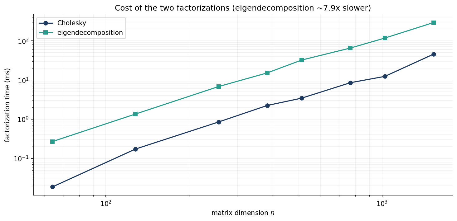
**Figure 1.** Wall-clock cost of the two factorizations against matrix dimension $n$, on log-log axes. Both scale like $n^3$, but Cholesky (navy) runs several times faster than the eigendecomposition (teal) across the whole range — the gap is a constant factor, not a change in slope.

The two lines are parallel — both are cubic in $n$ — but Cholesky sits consistently below, running roughly eight times faster on this machine. If your covariance is clean and you factorize it inside a hot loop, that constant is real money. Cholesky wins on cost, decisively.

When Cholesky Isn’t an Option

So why ever pay for the eigendecomposition? Because in practice $\Sigma$ is rarely handed to you clean. Correlation matrices are estimated, and estimated correlation matrices are routinely not positive definite: pairwise deletion with missing data, blending a model matrix with hand-set expert overrides, or an aggressive shrinkage step can each push the smallest eigenvalue just below zero. It does not take a dramatic defect — a rounding-scale negative eigenvalue is enough to stop Cholesky cold.

Python 3.13 — A Non-PD Correlation Matrix, and the Eigen Repair

import numpy as np
import matplotlib
matplotlib.use("Agg")
import matplotlib.pyplot as plt

NAVY, RED = "#1e3a5f", "#c0392b"

def expcorr(n, rho=0.6):
    i = np.arange(n)
    return rho ** np.abs(i[:, None] - i[None, :])

def bad_corr(n=10):
    # a valid (PD) correlation matrix lightly corrupted by a few inconsistent
    # "expert overrides" until one eigenvalue slips just below zero
    base = expcorr(n, 0.55)
    for seed in range(20000):
        rng = np.random.default_rng(seed)
        C = base.copy()
        for _ in range(3):
            i, j = rng.integers(0, n, size=2)
            if i == j:
                continue
            v = rng.uniform(-0.85, 0.85)
            C[i, j] = C[j, i] = v
        np.fill_diagonal(C, 1.0)
        w = np.linalg.eigvalsh(C)
        if -0.12 < w.min() < -0.02:                 # barely indefinite: the common trap
            return C, w
    raise RuntimeError("no indefinite matrix found")

C, w = bad_corr()

try:                                                # Cholesky route: stops outright
    np.linalg.cholesky(C)
    chol_ok = True
except np.linalg.LinAlgError:
    chol_ok = False

# eigen route: clip negatives to zero -> nearest PSD, renormalize to unit diagonal
wv, Q = np.linalg.eigh(C)
Cpsd = (Q * np.clip(wv, 0.0, None)) @ Q.T
d = np.sqrt(np.diag(Cpsd))
Cfix = Cpsd / np.outer(d, d)                        # repaired correlation matrix
wf, Qf = np.linalg.eigh(Cfix)
Afac = Qf * np.sqrt(np.clip(wf, 0.0, None))
rng = np.random.default_rng(0)
X = rng.standard_normal((200000, C.shape[0])) @ Afac.T
err = np.max(np.abs(np.corrcoef(X, rowvar=False) - Cfix))
print(f"cholesky succeeded: {chol_ok}   sampler max corr error: {err:.4f}")

ws = np.sort(w); idx = np.arange(1, len(w) + 1)
fig, ax = plt.subplots(figsize=(10, 5), facecolor="white")
ax.axhline(0, color="#888888", lw=1.0)
pos = ws >= 0
ax.vlines(idx[pos], 0, ws[pos], color=NAVY, lw=6, label="positive eigenvalues")
ax.vlines(idx[~pos], 0, ws[~pos], color=RED, lw=6, label="negative (Cholesky fails here)")
ax.plot(idx, ws, "o", color="#333333", ms=4)
ax.set_ylim(bottom=ws[0] - 0.35)
ax.annotate(r"$\lambda_{\min}$" + f" = {ws[0]:.3f} < 0" + "\nCholesky raises here",
            xy=(1, ws[0]), xytext=(2, 1),
            fontsize=10, color=RED, va="center",
            arrowprops=dict(arrowstyle="->", color=RED, lw=1.3))
ax.set_xlabel("eigenvalue index (sorted)")
ax.set_ylabel("eigenvalue")
ax.set_title("Spectrum of an estimated correlation matrix that is not positive definite")
ax.legend(framealpha=0.7, loc="upper left")
ax.spines[["top", "right"]].set_visible(False)
fig.tight_layout(pad=1.5)
fig.savefig("fig_2.png", dpi=150, bbox_inches="tight")

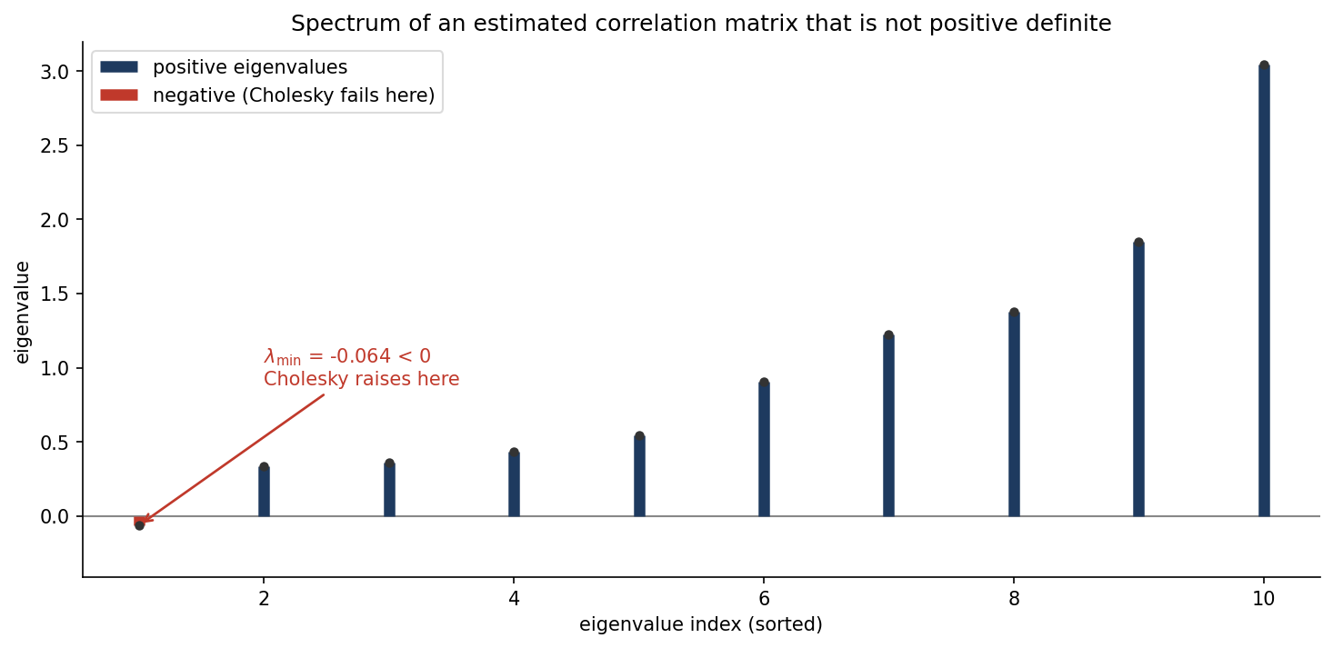
**Figure 2.** Sorted eigenvalues of a lightly corrupted correlation matrix. Nine are positive, but the smallest sits just below zero — a defect of about $-0.06$. That lone negative eigenvalue is enough for Cholesky to raise an error, while the eigendecomposition simply reports it.

Cholesky fails on this matrix. The eigendecomposition does not: because it exposes the spectrum, we can clip the negative eigenvalues to zero, rebuild the matrix, and renormalize the diagonal back to ones. The result is the closest positive-semidefinite correlation matrix in a rough sense — a one-line cousin of Higham’s nearest-correlation-matrix algorithm — and it is perfectly usable as a sampler. The check in the code confirms it: draws from the repaired matrix reproduce its correlations to within Monte Carlo noise.

The Rule, and the Hybrid

The two routes are not competitors so much as tools for two different situations:

$\Sigma$ is genuinely positive definite and you factor it often — use Cholesky. It is several times faster and numerically cleaner, and the robustness of the spectral route buys you nothing here.
$\Sigma$ is estimated and might be indefinite — use the eigendecomposition, clip, and sample. It degrades gracefully exactly where Cholesky stops dead.

In production you rarely have to choose in advance. The honest pattern is a hybrid: attempt the Cholesky, catch the failure, and fall back to the eigen-clip only when the matrix turns out to be broken. You pay the fast path’s price on every clean matrix and the safe path’s price only when you must — the speed of Cholesky with the survival instinct of the spectral method.

Working on a pricing model or risk system? Let’s talk.