Integrating Oscillations: Filon vs Levin

The Problem With Wiggles

Oscillatory integrals of the form $\int_a^b f(x)\,e^{i\omega x}\,dx$ punish naive quadrature. To resolve the $\omega/2\pi$ oscillations on the interval you need $O(\omega)$ sample points, and on any fixed grid the error of a Newton–Cotes rule does not decay as $\omega \to \infty$ — it wanders around $O(1)$. Two classical methods sidestep this entirely by handling the oscillation analytically rather than sampling it. This post pits them against each other on a problem with a known answer.

A Test With a Known Answer

We integrate a smooth amplitude against a pure oscillation:

$$I(\omega) = \int_0^1 e^{x}\, e^{i\omega x}\, dx = \frac{e^{\,1+i\omega} – 1}{1 + i\omega}$$

$(1)$

The closed form on the right lets us measure the true error at any frequency. The amplitude $e^{x}$ is analytic; all the difficulty lives in the factor $e^{i\omega x}$.

Filon: Integrate the Oscillation Exactly

Louis Filon’s idea (1928) is to split $\lbrack 0,1\rbrack$ into pairs of panels and, on each pair, replace only the amplitude $f$ by the quadratic through three nodes. The oscillatory factor $e^{i\omega x}$ is then integrated against that quadratic in closed form. The oscillation is never sampled — only the smooth part is approximated — so the cost is a fixed $2N+1$ nodes and the error is set by the piecewise-quadratic fit, essentially independent of $\omega$.

Levin: Turn the Integral Into an ODE

David Levin’s collocation method (1982) is slicker. Seek a function $p$ solving

$$p'(x) + i\omega\, p(x) = f(x)$$

$(2)$

Then $\big(p(x)\,e^{i\omega x}\big)’ = f(x)\,e^{i\omega x}$, and the fundamental theorem collapses the integral to boundary values:

$$I(\omega) = p(1)\,e^{i\omega} – p(0)$$

$(3)$

Approximate $p$ by a degree-$(n-1)$ polynomial and enforce the ODE at $n$ collocation points — one small linear solve, again with no sampling of the oscillation. The $i\omega\, p$ term dominates the diagonal, so the system becomes better conditioned as $\omega$ grows: the method likes high frequencies.

The Code

Both methods, the naive Simpson baseline, and the error sweep against the exact value:

Python 3.13 — Filon vs Levin Oscillatory Quadrature

import numpy as np
import matplotlib
matplotlib.use("Agg")
import matplotlib.pyplot as plt

def f(x):     return np.exp(x)                      # smooth amplitude
def exact(w): return (np.exp(1 + 1j*w) - 1)/(1 + 1j*w)

def simpson(w, N):                                  # naive baseline (same nodes as Filon)
    h = 1.0/(2*N); x = np.linspace(0, 1, 2*N+1)
    g = f(x)*np.exp(1j*w*x)
    return h/3*(g[0] + g[-1] + 4*np.sum(g[1::2]) + 2*np.sum(g[2:-1:2]))

def filon(w, N):                                    # amplitude -> quadratic, oscillation exact
    h = 1.0/(2*N); x = np.linspace(0, 1, 2*N+1); fx = f(x); th = w*h
    if abs(th) < 1e-3:                              # small-angle Taylor (avoid cancellation)
        al = 2*th**3/45; be = 2/3 + 2*th**2/15; ga = 4/3 - 2*th**2/15
    else:
        s, c = np.sin(th), np.cos(th)
        al = 1/th + np.sin(2*th)/(2*th**2) - 2*s**2/th**3
        be = 2*((1 + c**2)/th**2 - np.sin(2*th)/th**3)
        ga = 4*(s/th**3 - c/th**2)
    cwx, swx = np.cos(w*x), np.sin(w*x)
    Ce = np.sum(fx[0::2]*cwx[0::2]) - 0.5*(fx[0]*cwx[0] + fx[-1]*cwx[-1]); Co = np.sum(fx[1::2]*cwx[1::2])
    Ic = h*(al*(fx[-1]*swx[-1] - fx[0]*swx[0]) + be*Ce + ga*Co)
    Se = np.sum(fx[0::2]*swx[0::2]) - 0.5*(fx[0]*swx[0] + fx[-1]*swx[-1]); So = np.sum(fx[1::2]*swx[1::2])
    Is = h*(al*(fx[0]*cwx[0] - fx[-1]*cwx[-1]) + be*Se + ga*So)
    return Ic + 1j*Is

def levin(w, n):                                    # collocation: p' + i w p = f
    j = np.arange(n); xk = 0.5*(1 - np.cos(np.pi*(2*j+1)/(2*n)))   # Chebyshev nodes on [0,1]
    A = np.zeros((n, n), complex)
    for k in range(n):
        A[:, k] = ((k*xk**(k-1)) if k > 0 else np.zeros(n)) + 1j*w*xk**k
    c = np.linalg.solve(A, f(xk))
    p = lambda X: sum(c[k]*X**k for k in range(n))
    return p(1.0)*np.exp(1j*w) - p(0.0)

ws = np.linspace(1, 300, 200); floor = 1e-17
es = np.array([max(abs(simpson(w, 8) - exact(w)), floor) for w in ws])
ef = np.array([max(abs(filon(w, 8)   - exact(w)), floor) for w in ws])
el = np.array([max(abs(levin(w, 10)  - exact(w)), floor) for w in ws])

NAVY, TEAL, DANGER = "#1e3a5f", "#2a9d8f", "#c0392b"
fig, ax = plt.subplots(figsize=(10, 5), facecolor="white")
ax.semilogy(ws, es, color=DANGER, lw=1.2, ls="--", alpha=0.9, label="composite Simpson (naive, 17 nodes)")
ax.semilogy(ws, ef, color=NAVY, lw=1.5, label="Filon (17 nodes)")
ax.semilogy(ws, el, color=TEAL, lw=1.5, label="Levin collocation (10 nodes)")
ax.set_xlabel(r"frequency $\omega$")
ax.set_ylabel(r"absolute error $|I_{\mathrm{num}} - I_{\mathrm{exact}}|$")
ax.set_title(r"Oscillatory quadrature of $\int_0^1 e^x e^{i\omega x}\,dx$")
ax.legend(framealpha=0.7, loc="center right",
          bbox_to_anchor=(0.98, 1e-11), bbox_transform=ax.get_yaxis_transform())
ax.spines[["top", "right"]].set_visible(False)
fig.tight_layout(pad=1.5)
fig.savefig("fig_1.png", dpi=150, bbox_inches="tight")

**Figure 1.** Absolute error against the exact value as the frequency $\omega$ grows, all methods on a *fixed* node budget. Composite Simpson (red) drifts up to $O(1)$; Filon (navy) stays near $10^{-6}$; Levin (teal), with fewer nodes, sits near machine precision.

What the Error Says

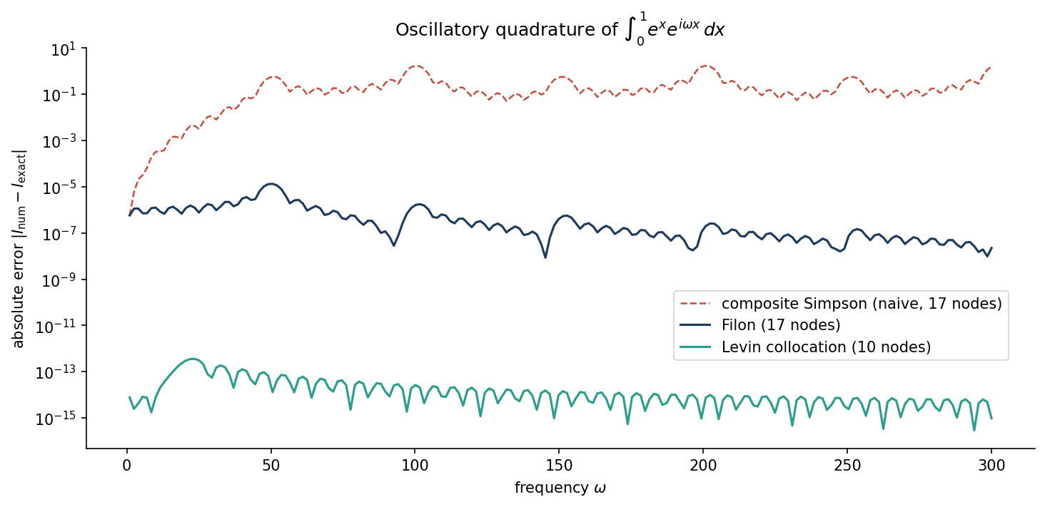
Three regimes, and all of them are real numbers off the plot above:

Composite Simpson (same 17 nodes as Filon) climbs to $O(1)$ — with a fixed grid it simply cannot follow the oscillation, and its error is worthless past $\omega \approx 20$.
Filon holds steady near $10^{-6}$, bounded across the whole frequency range and, if anything, improving slightly as $\omega$ grows. Its accuracy is capped by the piecewise-quadratic model of the amplitude, not by the frequency.
Levin sits at roughly $10^{-14}$ — machine precision — using fewer points (10 vs 17). Its global polynomial collocation resolves the analytic amplitude $e^{x}$ almost exactly, and the $i\omega$ diagonal keeps the linear system well conditioned at high $\omega$.

Takeaway

Both Filon and Levin do the one thing naive quadrature cannot: their error stays bounded — even shrinks — as the integrand oscillates faster. For a smooth amplitude on a single interval, Levin’s spectral collocation wins decisively and cheaply. Filon’s virtue is elsewhere: it is trivial to apply to piecewise or tabulated amplitudes, where a global polynomial fit is not available. The lesson is the same one that runs through all of numerical analysis — when part of your integrand is known exactly, integrate it exactly, and spend your samples only on the part you don’t know.

Need a reliable numerical implementation for your problem? Get in touch.