The Itô Integral: A Running Bet You Fix Before the Flip

The Idea in One Line

An Itô integral is not the area under a curve — it is a *running bet* whose size you must fix **before** each coin flip. That single constraint is the whole difference between ordinary calculus and stochastic calculus.

Why the Naive Guess Fails

If $W_t$ is Brownian motion, you might expect $\int_0^T W_t \, dW_t = \tfrac{1}{2} W_T^2$, copying the ordinary rule $\int x \, dx = \tfrac{1}{2} x^2$. It is wrong. The correct result carries a correction term:

$$\int_0^T W_t \, dW_t = \tfrac{1}{2} W_T^2 – \tfrac{1}{2} T$$

$(1)$

The extra $-\tfrac{1}{2} T$ is the accumulated quadratic variation — the price of randomness that ordinary calculus never had to pay.

A Ten-Line Check

We can watch the correction appear numerically. For a partition of $\lbrack 0, T\rbrack$ into $n$ steps we estimate $\tfrac{1}{2} W_T^2 – \sum_i W_{t_i}\,\Delta W_i$ across many Brownian paths and track it as $n$ grows.

Python 3.13 — Itô Correction Convergence

import numpy as np
import matplotlib
matplotlib.use("Agg")
import matplotlib.pyplot as plt

rng = np.random.default_rng(0)
T = 1.0
ns = [50, 100, 200, 500, 1000, 2000, 5000]
est = []
for n in ns:
    dt = T / n
    dW = rng.normal(0, np.sqrt(dt), size=(4000, n))
    W  = np.cumsum(dW, axis=1)
    Wm = np.concatenate([np.zeros((4000, 1)), W[:, :-1]], axis=1)
    ito  = (Wm * dW).sum(axis=1)          # Ito sum
    corr = 0.5 * W[:, -1]**2 - ito         # -> 1/2 * T
    est.append(corr.mean())

NAVY, TEAL = "#1e3a5f", "#2a9d8f"
fig, ax = plt.subplots(figsize=(10, 5), facecolor="white")
ax.plot(ns, est, "o-", color=NAVY, lw=1.5, label=r"Monte-Carlo estimate")
ax.axhline(0.5 * T, color=TEAL, lw=1.0, ls="--", alpha=0.8, label=r"theory: $T/2$")
ax.set_xscale("log")
ax.set_xlabel("partition size $n$")
ax.set_ylabel("correction term")
ax.set_title("The Ito correction converges to T/2")
ax.legend(framealpha=0.7)
ax.spines[["top", "right"]].set_visible(False)
fig.tight_layout(pad=1.5)
fig.savefig("fig_1.png", dpi=150, bbox_inches="tight")

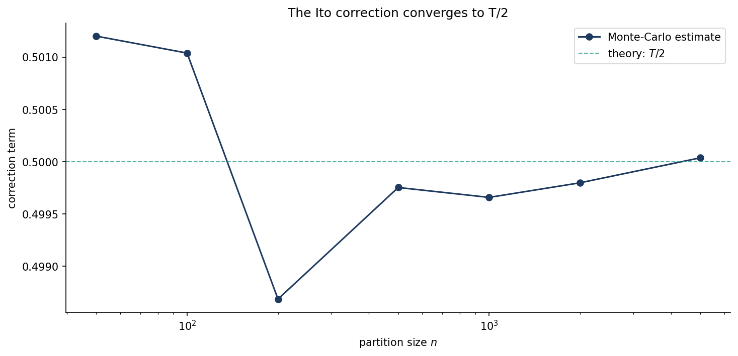
**Figure 1.** Monte-Carlo estimate of $\tfrac{1}{2} W_T^2 – \int_0^T W_t \, dW_t$ against partition size $n$. As the mesh refines, the estimate settles onto the theoretical value $T/2$.

The estimate settles onto $\tfrac{1}{2} T$ — the correction is real, and it is exactly the accumulated quadratic variation.

Why It Matters

Every pricing model that discounts a hedged portfolio leans on this correction. Drop it and your option prices drift; keep it and the risk-neutral machinery closes. In a world with quadratic variation you cannot look one instant into the future — and that single honesty is what makes the mathematics of finance both hard and true.

Working on a pricing model or risk system? Let’s talk.