
The Average That Drowned a City
Forty-Nine Feet
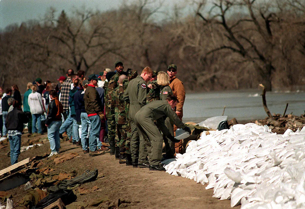
In February 1997 the National Weather Service told Grand Forks, North Dakota, that the Red River of the North would crest at 49 feet that spring. The city and its neighbour across the river, East Grand Forks, Minnesota, built their dikes to about 52 feet, three feet of margin above the number, with some 3.5 million sandbags.
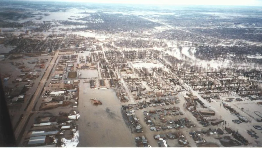
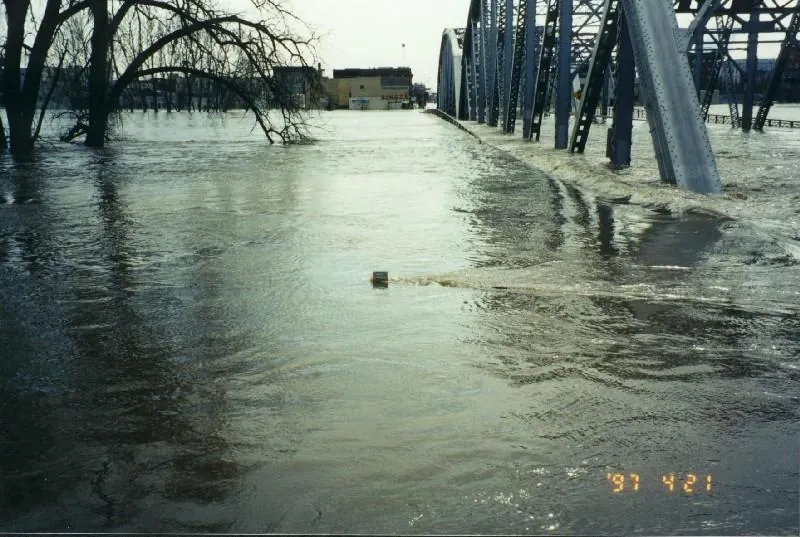
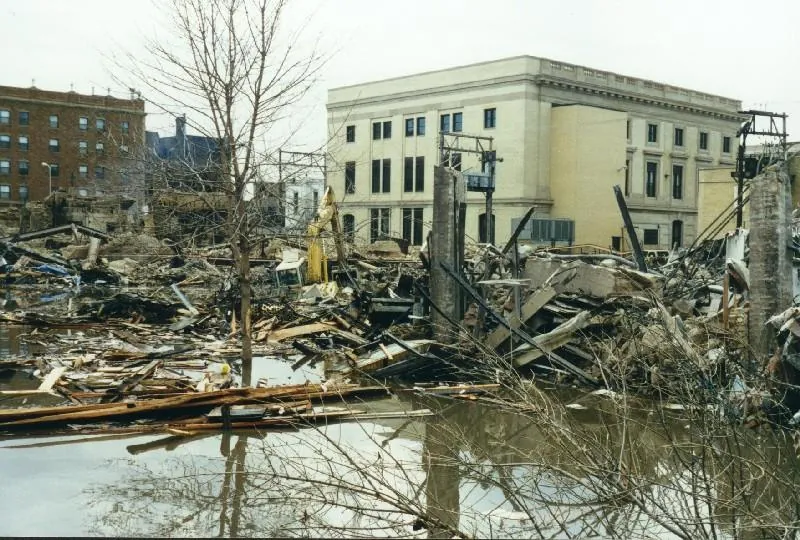
On 18 April the dikes began to fail. The river crested at 54.35 feet. More than 50,000 people were evacuated, three quarters of Grand Forks and all of East Grand Forks. Downtown caught fire while it stood in floodwater, and eleven buildings burned. The losses ran to over $2 billion. Not one person died in the flood itself. A resident’s ruined house carried the verdict: 49 feet my ass.
This post is about one line of mathematics, and it is not subtle: Grand Forks prepared for the damage of the average crest, and what it needed to prepare for was the average damage. The first is zero. The second was not. The difference between the two has a name, and a date: Jensen’s inequality, 1906.
The Number Was a Median
The 49 feet was never a ceiling. The Weather Service’s own assessment of the flood, published in 1998, says its spring outlooks that assume normal future precipitation “are approximately at the median; i.e., they have approximately a 50 percent chance of being equaled or exceeded.” The number the city built to was a coin toss.
The outlook came as two numbers: 47.5 feet assuming no more precipitation, 49 feet assuming normal precipitation. The same assessment found that “many users interpreted the two flood crest levels issued in the outlook as a range; i.e., the two were viewed as minimum and maximum levels,” and that repeating the same value all spring produced a “locking in” on 49 feet. Worse, 49 feet was only 0.2 foot above the record of 1979, which the city had survived, so “rather than elevating concern, the 49-foot outlook actually created a sense of complacency.”
The forecaster’s track record was public. From 1980 to 1997 the Weather Service issued twelve spring outlooks for East Grand Forks, and the crest that came equalled or beat the outlook in six of them. Before 1997 it had happened in five years out of eleven. Its misses ran from 9.2 feet too high to 4.3 feet too low.
Jensen’s Inequality, at Fifty-Two Feet
Write $H$ for the crest, uncertain in February, and measure the damage as the depth of water over the dikes:
$D$ is convex: flat at zero below the dikes, rising beyond them. For any convex function, Jensen’s inequality says the average of the function is at least the function of the average, and strictly more whenever the uncertainty reaches the place where the function bends. Here it bends at 52 feet.
The city’s arithmetic was the right-hand side. Plug the forecast crest into the damage: $D(49) = 0$. Nothing to fear. The quantity that mattered was the left-hand side: the damage averaged over every crest the forecast still allowed. That is not zero, and the forecaster’s own record says how far from zero it was.
Take the Weather Service at its word that the outlook was the median, and take its typical miss from its record: the root mean square of its eleven misses before 1997 is 4.5 feet. Then the expected depth over the dikes has a closed form,
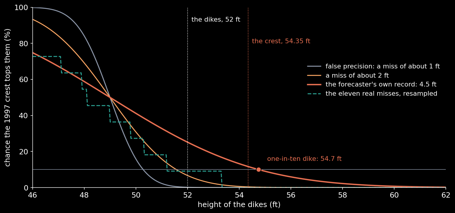
with $\mu = 49$ feet, $\sigma = 4.5$ feet and dikes at $L = 52$ feet. It comes to 0.67 foot, against the forecast’s zero. The chance that the crest would top the dikes at all was 25%: one in four. Drop the normal shape and simply replay the eleven real misses on top of 49 feet, and one of them (1989, when the river beat the outlook by 4.3 feet) clears the dikes: one in eleven, because the outlooks had more often erred high than low. One in four or one in eleven. Not zero.
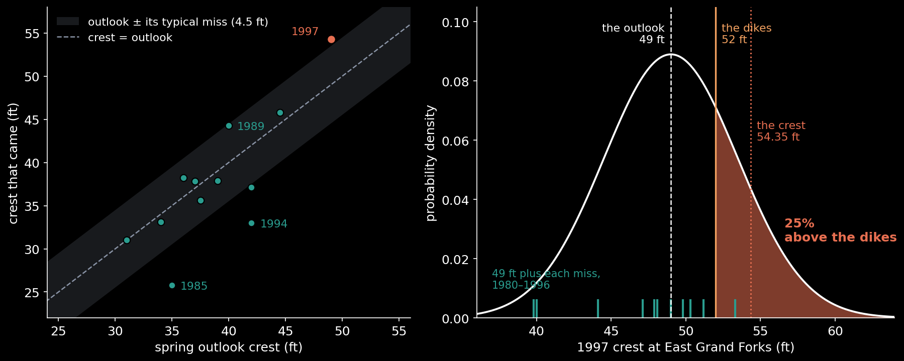
The river came in at 54.35 feet, 1.2 typical misses above the outlook. Nothing about that crest was outside the forecast’s own record. The National Research Council said so plainly in 2006: the actual crest “was within the error range one would expect for such a forecast which could have been, but was not, communicated along with the forecast.”
The Gap Is the Variance
Swapping $\mathbb{E}[f(X)]$ for $f(\mathbb{E}[X])$ is the beginner’s version of this mistake. Grand Forks shows the version that costs billions. Expand any smooth $f$ around the mean:
Jensen’s gap is curvature times variance. The curvature is a property of the city: where its dikes stand, what lies behind them. The variance is a property of the forecast. A single number has a variance of zero, and with zero variance Jensen’s gap is exactly zero, whatever the curvature. A number published without its spread does not report a wrong average; it reports no uncertainty at all, and the arithmetic that follows inherits the zero. The Weather Service’s own finding was that “many users developed a false sense of precision.”
The size of the variance is not a detail. With the same 49-foot median and the same dikes, a typical miss of one foot puts the chance of overtopping at one in a thousand; two feet, about seven in a hundred; the record’s four and a half feet, one in four. Read the median with a spread that is too narrow, and you have made the mistake as surely as if you had ignored the spread altogether. Sam Savage, who has spent a career collecting these, calls the whole family the flaw of averages.
The decision was there to be made. Ken Vein, the Grand Forks city engineer, said afterwards: “With proper advance notice we could have protected the city to almost any elevation.” Asked for dikes with only a one-in-ten chance of being topped, the forecaster’s own record answers 54.7 feet: above the crest that came.
This is the code that does all of it, from the Weather Service’s own table:
Python 3.13 — The Grand Forks Outlook, Averaged Properly
import numpy as np
from math import erf, exp, pi, sqrt

# NWS outlook crest (normal future precipitation) and the crest that came,
# East Grand Forks, from the NWS's own 1998 service assessment, Table 3
record = {1980: (31.0, 31.0), 1982: (42.0, 37.1), 1984: (36.0, 38.2),
          1985: (35.0, 25.8), 1986: (39.0, 37.9), 1987: (34.0, 33.1),
          1989: (40.0, 44.3), 1993: (37.5, 35.6), 1994: (42.0, 33.0),
          1995: (37.0, 37.8), 1996: (44.5, 45.8)}       # all known by 1997
forecast, dikes = 49.0, 52.0

miss = np.array([crest - outlook for outlook, crest in record.values()])
s = sqrt((miss**2).mean())                           # the typical miss
Phi = lambda z: 0.5 * (1 + erf(z / sqrt(2)))
phi = lambda z: exp(-z * z / 2) / sqrt(2 * pi)

def damage(h):                       # feet of water over the dikes: convex
    return max(0.0, h - dikes)

def expected_damage(sigma):          # E[damage(H)], H ~ N(forecast, sigma^2)
    z = (dikes - forecast) / sigma
    return sigma * phi(z) - (dikes - forecast) * (1 - Phi(z))

print(f"outlook met or beaten: {(miss >= 0).sum()} of {len(miss)} years")
print(f"typical miss: {s:.2f} ft")
print(f"damage at the forecast, D(E[H]): {damage(forecast):.2f} ft")
print(f"expected damage, E[D(H)]: {expected_damage(s):.2f} ft")
print(f"chance the crest tops the dikes: {1 - Phi((dikes - forecast) / s):.0%}")
as_they_were = (forecast + miss > dikes).mean()       # no distribution assumed
print(f"  the eleven real misses as they were: {as_they_were:.0%}")
print(f"dikes for a one-in-ten chance: {forecast + 1.2816 * s:.1f} ft")
for sigma in (1.0, 2.0, s):          # the variance is the whole Jensen gap
    print(f"  if the typical miss were {sigma:.1f} ft: "
          f"tops the dikes {1 - Phi((dikes - forecast) / sigma):.1%}")

# outlook met or beaten: 5 of 11 years
# typical miss: 4.48 ft
# damage at the forecast, D(E[H]): 0.00 ft
# expected damage, E[D(H)]: 0.67 ft
# chance the crest tops the dikes: 25%
#   the eleven real misses as they were: 9%
# dikes for a one-in-ten chance: 54.7 ft
#   if the typical miss were 1.0 ft: tops the dikes 0.1%
#   if the typical miss were 2.0 ft: tops the dikes 6.7%
#   if the typical miss were 4.5 ft: tops the dikes 25.2%
After the Water
The Weather Service’s assessment recommended conveying the uncertainty of its outlooks “explicitly and objectively,” and the spring outlooks for the Red River are now given as chances of exceeding each level, not as one number to build to. Grand Forks rebuilt behind permanent levees and floodwalls.
The 49 feet was not a bad forecast. It was a median, and it said so in the small print. The mistake was to put a median into a convex loss and read off the answer, which is the oldest mistake in probability. Jensen wrote it down in 1906: the damage of the average is not the average damage. In Grand Forks the difference was a city.
Sources
- National Weather Service, Red River of the North 1997 Floods: Service Assessment and Hydraulic Analysis, U.S. Department of Commerce, National Oceanic and Atmospheric Administration (August 1998).
- Wikipedia, “1997 Red River flood in the United States” (accessed 30 September 2026), for the evacuation, the fire and the sandbags.
- R. A. Pielke Jr., “Who decides? Forecasts and responsibilities in the 1997 Red River flood”, Applied Behavioral Science Review 7 (1999) 83–101.
- J. L. W. V. Jensen, “Sur les fonctions convexes et les inégalités entre les valeurs moyennes”, Acta Mathematica 30 (1906) 175–193.
- National Research Council, Completing the Forecast: Characterizing and Communicating Uncertainty for Better Decisions Using Weather and Climate Forecasts, National Academies Press (2006).
- S. L. Savage, The Flaw of Averages: Why We Underestimate Risk in the Face of Uncertainty, Wiley (2009).
Every number in the text and both charts are computed by the scripts archived with this post, from the Weather Service’s own table of outlooks and crests (Table 3 of source 1). The photographs are works of the United States government, in the public domain.
Interested in applying these ideas to your work? Get in touch.