The Cube Root That Runs the Treasury

Every Morning at Nine

A company’s treasurer makes the same small decision every morning: how much of the company’s money to leave in the bank
account, where it earns nothing but pays the bills, and how much to move into short-term securities, where it earns
interest but costs a fee every time it moves. Hold too much cash and the interest is lost. Hold too little and the
transfers pile up. In 1966 Merton Miller, who would later share a Nobel prize, and Daniel Orr worked out the best rule.
It is a band set by three numbers, and the one that matters is a cube root.

**Figure 1.** An antique cash register. The question it raises is older than the machine: how much money to keep at hand, and how much to put to work. Photograph by Erik Mclean, Pexels.

A Random Walk in the Bank Account

Money arrives and leaves every day, and the net flow is hard to predict: a customer pays early, a supplier’s invoice
lands, payroll goes out. Miller and Orr modelled the cash balance as a Brownian motion with no drift and a variance of
$\sigma^2$ a day, and priced its two costs: a fixed fee $F$ for every transfer between cash and securities, and the
interest $r$ a day forgone on every dollar held as cash. William Baumol had solved the version with a steady, known
outflow in 1952, and his answer was a square root. With a random flow the answer changes shape.

The rule they studied has three levels: a lower limit $L$, set by the bank or the board; a return point $L + z$; and an
upper limit $L + h$. Inside the band, do nothing. When the balance falls to $L$, sell securities to bring it up to
$L + z$. When it rises to $L + h$, invest the excess down to $L + z$. This is impulse control of a diffusion: the
treasurer acts in jumps, only at the edges, and leaves the random walk alone in between. Two facts about a Brownian motion
in an interval price the whole rule. It takes $z(h-z)/\sigma^2$ days on average to leave the band from the return point,
and while inside it sits, on average, $(h+z)/3$ above the lower limit. The cost a day is then

$$C(z, h) = \frac{F\,\sigma^{2}}{z\,(h – z)} + \frac{r\,(h + z)}{3}$$

$(1)$

The first term is the transfer fees; the second is the interest lost on the average balance.

The Cube Root

Setting both derivatives to zero gives the rule:

$$h^{*} = 3\,z^{*}, \qquad z^{*} = \left(\frac{3\,F\,\sigma^{2}}{4\,r}\right)^{1/3}, \qquad C^{*} = 2\,r\,z^{*}$$

$(2)$

The return point sits a third of the way up the band, not in the middle. Cash near the bottom costs less interest than
cash near the top, so the band leans low. And at the optimum the interest lost is always exactly twice the fees paid.

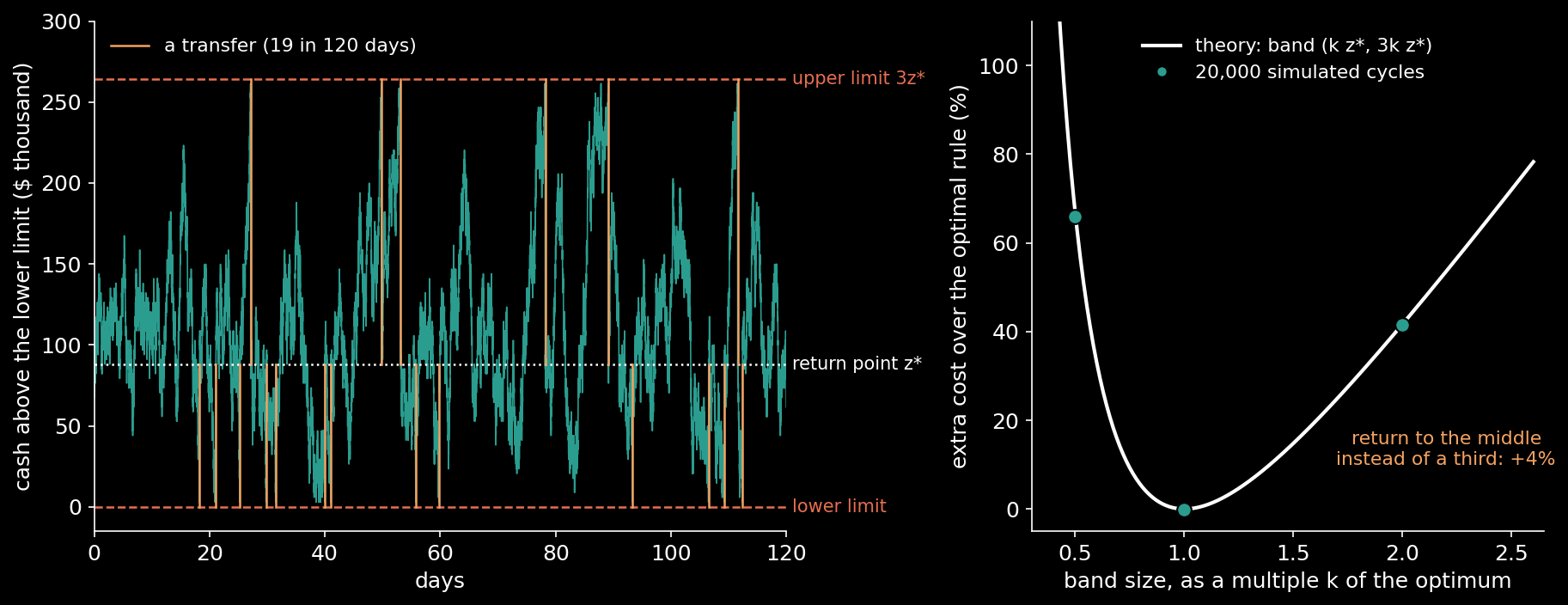
Take a firm whose daily net cash flow has a standard deviation of $50,000, which pays $50 for each transfer and could earn
5% a year on money not held as cash. Its return point is $88,000 above the lower limit and its upper limit $264,000. The
balance averages $117,500, a transfer happens every 6.2 days, 59 times a year, and the whole policy costs about $8,800 a
year: $5,900 of interest forgone and $2,900 of fees.

Left: 120 simulated days of the example firm's cash under the rule. It wanders freely inside the band, and each orange line is a transfer back to the return point, 19 of them. Right: the extra cost of a band of the wrong size, in theory (line) and over 20,000 simulated cash cycles each (dots). The… — **Figure 2.** Left: 120 simulated days of the example firm’s cash under the rule. It wanders freely inside the band, and each orange line is a transfer back to the return point, 19 of them. Right: the extra cost of a band of the wrong size, in theory (line) and over 20,000 simulated cash cycles each (dots). The bottom of the curve is flat.

Algorithm — The Miller–Orr Rule for a Cash Balance

input:  F        cost of one transfer
        sigma2   variance of the daily net cash flow
        r        interest a day on money moved to securities
        L        the lowest balance allowed
z   <- (3 F sigma2 / (4 r))^(1/3)       the return point, above L
h   <- 3 z                              the upper limit, above L
every day, with cash X:
    if X <= L:        sell securities worth L + z - X
    if X >= L + h:    buy securities worth X - (L + z)
    otherwise:        do nothing
expect: average cash L + 4z/3, a transfer every 2 z^2 / sigma2 days,
        total cost 2 r z a day

Why a Cube Root Forgives

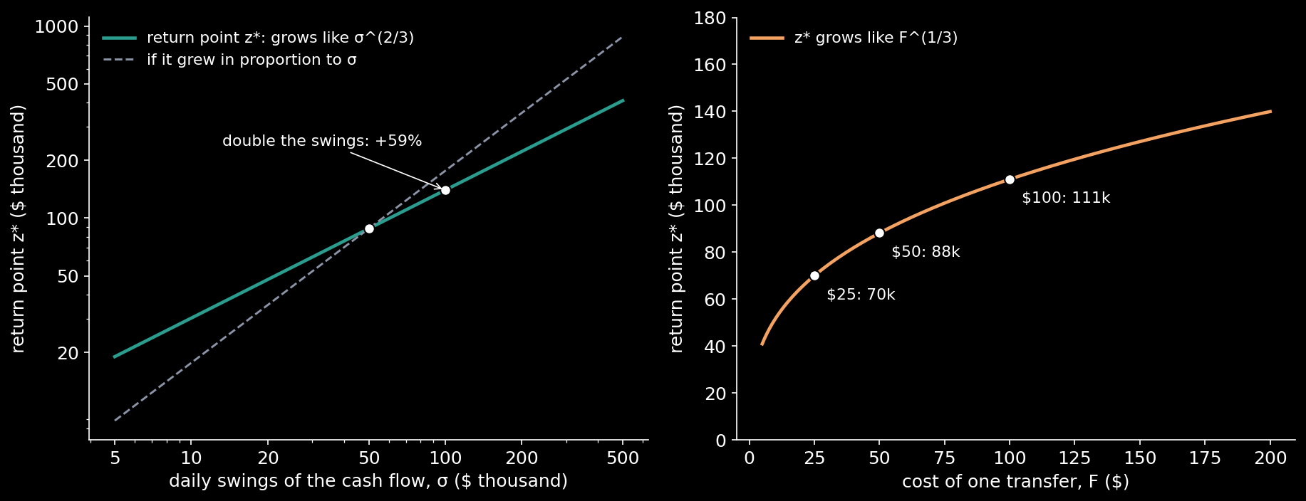
The return point grows like $\sigma^{2/3}F^{1/3}r^{-1/3}$, and those small exponents make the rule remarkably tolerant.
Double the day-to-day swings of the cash flow and the buffer grows by only 59%; multiply them by ten and it grows 4.6
times. Halve the fee for a transfer and the buffer shrinks by only 21%. A treasurer who reads a volatility estimate off
last quarter’s statements, and gets it somewhat wrong, still lands close to the right band.

The cost is just as forgiving near the optimum. A band a quarter too wide costs under 5% more. Returning to the middle of
the band instead of a third of the way up costs 4% more. Only gross errors are expensive: a band twice as wide as it
should be costs 42% more, and one half as wide costs 67% more, because transfers then come every day and a half.

**Figure 3.** Left: the return point against the daily swings of the cash flow, on log scales. It grows like the two-thirds power (teal), much more slowly than in proportion (dashed): doubling the swings adds 59%. Right: the return point against the cost of one transfer, which enters only as a cube root.

What the Rule Leaves Out

The model has no drift, and real cash flows have a calendar: payroll on Fridays, taxes each quarter. The later
mathematics of impulse control confirmed that a band is the right shape of policy far beyond their assumptions, drift
included. A fee proportional to the amount moved, rather than fixed, changes
the answer: the treasurer then trims the balance back to the edge of the band, just inside it, instead of jumping to a
return point. And a firm that faces a penalty for running out of cash sets its lower limit with that penalty in mind,
which the rule takes as given.

**Figure 4.** A vault lined with lockboxes. The mathematics of the band says to leave the money alone most of the time, and to know exactly where the edges are. Photograph by Ehtiram Mammadov, Pexels.

The treasurer who follows the rule does nothing on most mornings. That is not idleness. It is the optimal policy for a
random walk with a fixed cost of acting: watch, wait, and move only at the edges.

Sources

W. J. Baumol, “The transactions demand for cash: an inventory theoretic approach”, The Quarterly Journal of Economics 66 (1952) 545–556.
M. H. Miller and D. Orr, “A model of the demand for money by firms”, The Quarterly Journal of Economics 80 (1966) 413–435.
G. M. Constantinides and S. F. Richard, “Existence of optimal simple policies for discounted-cost inventory and cash management in continuous time”, Operations Research 26 (1978) 620–636.
J. M. Harrison, T. M. Sellke and A. J. Taylor, “Impulse control of Brownian motion”, Mathematics of Operations Research 8 (1983) 454–466.

Every number in the text and both charts are computed by the scripts archived with this post: the closed forms, each checked against a simulation of 20,000 cash cycles per policy, saved once. The example firm’s figures are an illustration, not a company’s accounts.

Interested in applying these ideas to your work? Get in touch.