
Reject Three Out of Four
No, Three Times in Four
In 2007 Frank Smets and Rafael Wouters published a model of the American economy built on 36 numbers that cannot be observed and had to be estimated: how sticky prices and wages are, how slowly habits change, how hard the central bank leans against inflation, how long each kind of shock lingers. They did not solve for those numbers. They let a random walk wander through all 36 at once, for 250,000 steps, and kept a record of where it went. In a footnote they report that the walk turned down 65% of the moves it proposed.
That is not a malfunction. It is close to the design. Dynare, the free software that central banks, finance ministries and international organisations use for this kind of model, tells its users to tune the walk until between a quarter and a third of its proposals are accepted, and its default step comes from a theorem published in 1997. The theorem says the best acceptance rate is 23.4%: the best walk turns down about three proposals in four. A walk that feels safe, accepting nine in ten, needs 23 times as many steps to learn the same thing.
The number comes from stochastic analysis. As the number of dimensions grows, the walk stops behaving like a walk and becomes a diffusion: a particle pushed up the slope of the probability and shaken by noise. 23.4% is where that diffusion runs fastest. This post follows it in four steps: the walk that says no, the diffusion it turns into, the acceptance rate where the diffusion is fastest, and the price of a timid walk. Then where the number runs, and why the field moved on to walks that use the slope.
The Walk That Says No
The walk was published in 1953 by five people at Los Alamos: Nicholas Metropolis, Arianna and Marshall Rosenbluth, and Augusta and Edward Teller. They wanted averages over the positions of many particles, rigid spheres in two dimensions, computed on the laboratory’s MANIAC computer. Averaging over every arrangement is hopeless, and drawing arrangements at random wastes almost every draw on ones that nature never visits. Their answer was to walk: from the current arrangement $x$, propose a nearby one $y$, and decide whether to go.
The last line is the whole trick. The flow from $x$ to $y$ equals the flow back, so once the walk is spread out like $\pi$ it stays spread out like $\pi$, and the share of time it spends anywhere is the probability there. A move uphill in probability is always taken; a move downhill is taken only sometimes. And a refusal is not wasted: staying put and counting $x$ again is exactly what keeps the books balanced. In Bayesian statistics $\pi$ is the posterior, the probability of the parameters given the data, and the walk’s record is a sample from it. That is how Smets and Wouters got their 36 numbers, with error bars.
Everything then turns on one dial, the step size $\ell$. Take tiny steps and almost every proposal is accepted, but the walk shuffles in place. Take huge steps and the walk stands still, because nearly every proposal lands somewhere improbable and is refused. Somewhere in between is the fastest walk. The $1/\sqrt d$ in the step is forced: in $d$ dimensions a move changes $\log\pi$ by a sum of $d$ terms, and unless each coordinate’s step shrinks like $1/\sqrt d$, that sum grows until every proposal is refused.
The Walk Becomes a Diffusion
In 1997 Gareth Roberts, Andrew Gelman and Walter Gilks asked what one coordinate of this walk looks like when the target is a product of $d$ identical pieces, $\pi(x) = \prod_i f(x_i)$, and time is counted in units of $d$ steps. Their answer is a theorem. As $d$ grows, the coordinate converges to a Langevin diffusion:
The drift pushes the coordinate up the slope of $\log f$, the noise shakes it, and the second line says that $f$ is the diffusion’s stationary density: $\mathscr{L}$ is its generator, and $\mathscr{L}^* f = 0$ is the Fokker–Planck equation at rest. That much would hold at any speed. What the walk decides is the speed $h(\ell)$, the single number in front of both terms. Run the same diffusion at twice the speed and it explores in half the time.
The speed comes from the acceptance rate. When the walk proposes a move, the log of $\pi(y)/\pi(x)$ is a sum of $d$ small, nearly independent terms, so by the central limit theorem it is Gaussian:
The mean is minus half the variance for a reason. When the walk is spread out like $\pi$, the average of $\pi(y)/\pi(x) = e^W$ is exactly 1, and a lognormal with mean 1 must have $\mathbb{E}W = -\tfrac12\operatorname{Var}W$. The speed is then plain bookkeeping: an accepted step moves a coordinate a squared distance of about $\ell^2/d$, a unit of time holds $d$ steps, and a fraction $a(\ell)$ of them are accepted.
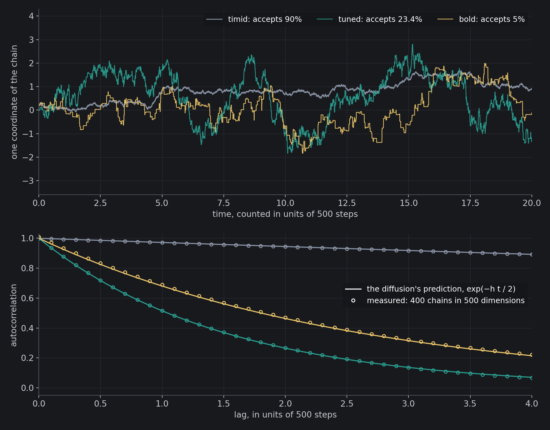
I checked the theorem on walks in 500 dimensions with a Gaussian $f$, where the limit is an Ornstein–Uhlenbeck process whose autocorrelation after time $t$ is $e^{-ht/2}$. At the three step sizes in the figure, the walks accepted 90.0%, 23.4% and 5.1% of their proposals (the limit says 90.0%, 23.4% and 5.0%), and their autocorrelations stay within 0.009 of the prediction at every lag.
23.4%
Write the speed in terms of the acceptance rate instead of the step, and the target drops out:
$I$ only scales the curve, so its peak sits at the same acceptance rate for every target of this kind, “under quite general conditions”, as the paper puts it. That is what makes the theorem useful. Tuning the step to the target is hard, because you do not know the target; tuning it to the acceptance rate is easy, because the walk counts its own refusals. The paper’s own advice is to tune the proposal so that the average acceptance rate is roughly 1/4.
I ran the walk on Gaussian targets in 1, 5, 20 and 100 dimensions and on the flatter-topped $f \propto e^{-x^4/4}$ in 100, started in equilibrium: 4,000 walks of 300 steps at each of 44 step sizes. From 20 dimensions on, the measured speeds fall on the one curve. The peak sits at 25.0% in 20 dimensions, 24.5% in 100 and 23.9% for the flatter-topped target; at 28.6% in 5 dimensions; and at 43.8% in one dimension, the 0.44 that Gelman, Roberts and Gilks had found for one dimension the year before.
The two ways to get it wrong do not cost the same. In the limit, a walk tuned to accept 5% needs 1.73 times the steps of the best one, and a walk at 10% needs 1.23 times. On the other side the curve falls away: 3.2 times the steps at 70%, 23 times at 90% and 89 times at 95%. Being too bold costs little. Being too careful is ruinous, because the steps that are almost always accepted are the steps that hardly move.
![The speed of a random walk against its acceptance rate. The white curve is the limit, the same for every target: 4a[Φ⁻¹(a/2)]². The circles are walks measured on Gaussian targets in 1, 5, 20 and 100 dimensions, and the diamonds on exp(−x⁴/4) in 100, each speed multiplied by the target's I. The…](https://zamrik.com/wp-content/uploads/blog/reject-three-out-of-four_fig_3.png)
The Price of Feeling Safe
Now a posterior with an answer. I built one with 36 parameters, the number Smets and Wouters estimated, correlated with each other and on scales from 0.01 to 3. It is Gaussian, so every posterior mean is known exactly. The walk’s proposals were shaped like the posterior, as they are in practice, and at each of 15 acceptance rates I ran 2,000 independent walks of 50,000 steps and measured how far each walk’s average of each parameter landed from the truth. The spread of those errors says how many independent draws the walk was worth.
At the tuned step, which accepted 24.2% of proposals in 36 dimensions, every 10,000 steps were worth 90 independent draws; the limit says 92. At 90% accepted they were worth 4.0, against 3.9 from the limit: 22 times fewer. To pin one parameter’s posterior mean to within a hundredth of its posterior standard deviation, the tuned walk needs about 1.1 million steps and the timid one about 25 million. The best of the 15 rates measured was 20.8%, at 91 draws, and a parabola through the top of the measured curve puts its peak at 23.9%.
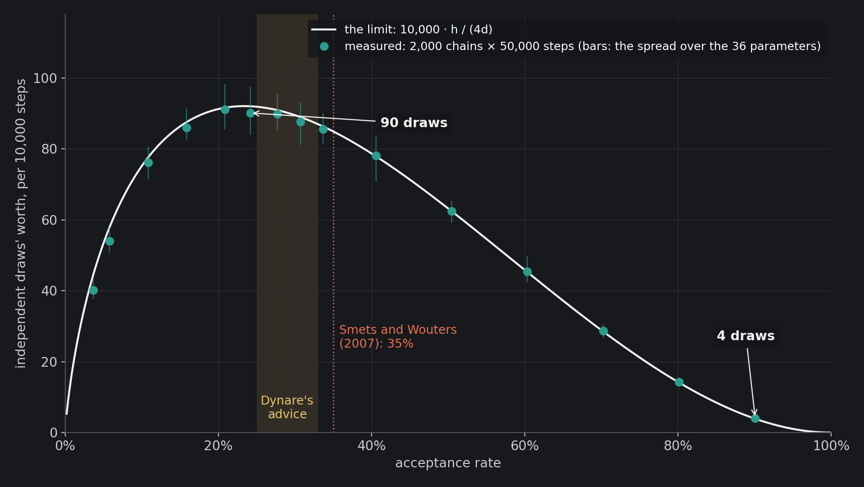
Smets and Wouters accepted 35% of proposals, and Dynare’s manual asks for 25% to 33%, with its automatic tuner aiming at 33%. Both sit on the flat top of the curve. In the limit, 35% costs 1.08 times the steps of the best and 33% costs 1.06 times; in the 36-parameter test, the walk that accepted 33.6% was worth 86 draws per 10,000 steps against 90 for the tuned one. The footnote can even be checked against the theorem. It says a step size of 0.3 gave a rejection rate of 0.65. If that step multiplies the posterior’s standard deviations, as Dynare’s does, it is $\ell = 0.3\sqrt{36} = 1.8$ in the units of this post, where the limit predicts 36.8% accepted. They saw 35%. Dynare’s default step is now the theorem itself: $2.38/\sqrt n$ for a model with $n$ parameters.
Where the Number Runs
The same rule, and often the same constant, is built into the software of other sciences.
In 2014 Nuno Faria and thirteen colleagues traced the HIV pandemic to its start. From viral sequences sampled across the Congo River basin they reconstructed the virus’s family tree, dated its branches, and placed the common ancestor of the pandemic strain, group M, around 1920 (95% credible interval 1909 to 1930), with Kinshasa as the focus of its early spread. The tree was sampled by a random walk in BEAST, version 1.8.0, in at least three chains of 250 million steps. BEAST’s moves tune themselves as they run, and the acceptance rate they aim at by default is 0.234.
The Planck collaboration’s final parameters of the universe, from its maps of the cosmic microwave background, include its age: 13.787 ± 0.020 billion years, when Planck’s data are combined with baryon acoustic oscillations measured in galaxy surveys. The constraints were computed with CosmoMC, whose author notes that scaling its proposals by about 2.4 is optimal when the target is Gaussian, the constant of the theorem, and that scalings of 1.5 to 2.5 work well, with acceptance rates of 0.2 to 0.5.
And samplers that learn their own proposals start from the same place: the adaptive Metropolis algorithm of Heikki Haario, Eero Saksman and Johanna Tamminen (2001) scales the covariance it has learned by $2.4^2/d$, a value it takes from Gelman, Roberts and Gilks.
Why Everyone Moved to the Slope
The theorem also says what the random walk costs as problems grow. Its step must shrink like $1/\sqrt d$, so crossing the target takes a number of steps that grows like $d$. A walk that uses the slope of $\log\pi$ does better. The Metropolis-adjusted Langevin algorithm proposes a move along one step of the Langevin diffusion itself, then accepts or refuses it by the same kind of rule:
Roberts and Jeffrey Rosenthal proved the Langevin line in 1998 by the same route, a diffusion limit, with the step shrinking like $d^{-1/6}$. Hamiltonian Monte Carlo was invented in 1987 by Duane, Kennedy, Pendleton and Roweth for lattice field theory, and in 2013 Beskos and four colleagues found its 0.651 and its $d^{1/4}$. Going from 100 parameters to a million multiplies the steps needed by 10,000 for the random walk, by 21.5 with Langevin steps and by 10 with Hamiltonian ones. That arithmetic is behind the move of Bayesian software, Stan among it, to Hamiltonian steps.
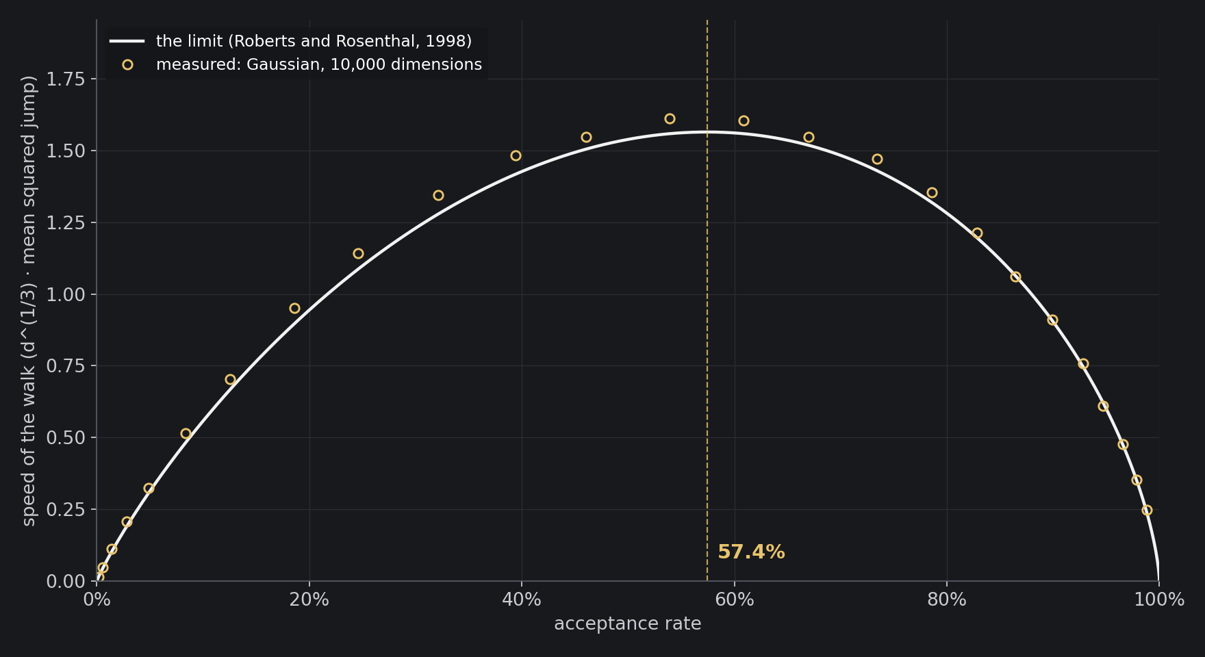
In 10,000 dimensions the Langevin walk’s measured acceptance rates agree with the limit to within 0.006 at every step size. Its measured speed runs between 0.3% and 7% above the limit, more at larger steps, because each step also carries the drift, a term the limit drops; the measured peak is at 56.5%.
Try It
The board runs the walk live in your browser, on a Gaussian target. Set the number of dimensions and the step size, or press a button for the timid, the half, the tuned and the bold walk, and watch it move on two of its coordinates, with its refusals marked, and on the diffusion’s clock. The cards computed from the limit (the acceptance rate, the speed, the steps needed against the best and the independent draws per 10,000 steps) were read back in a browser at nine settings and compared with Python’s numbers: all nine matched. The live walk, at 500 dimensions and the tuned step, accepted 22.9% of 15,939 proposals.
Algorithm — Tuning a Random-Walk Sampler to 23.4%
input:  log density log π on ℝᵈ, a start x, a first step size ℓ₀
log ℓ ← log ℓ₀;  lx ← log π(x)
for k = 1, 2, …
    y ← x + (ℓ/√d) Z,  Z ~ N(0, I_d)
        (in practice (ℓ/√d) L Z, with L Lᵀ ≈ the posterior's covariance)
    α ← min(1, exp(log π(y) − lx))
    with probability α:  x ← y;  lx ← log π(y)
    record x                       (a refusal records x again)
    log ℓ ← log ℓ + k^(−0.6) (α − 0.234)
        (Robbins–Monro: the corrections shrink, so the tuning settles)
check: from ℓ₀ = 0.1 in 100 dimensions, ℓ = 2.11 after 100 steps and 2.37
    on average over the last 20,000 of 40,000, accepting 23.40%;
    the theorem says 2.38 and 23.4%
check: d · (mean squared jump) against the acceptance rate,
    4,000 walks at each of 44 step sizes
check: the autocorrelation against exp(−h t / 2), 400 walks in 500 dimensions
check: a 36-parameter Gaussian posterior with a known answer,
    2,000 walks of 50,000 steps
The Name on the Algorithm
The method is called the Metropolis algorithm. Invited to a conference at Los Alamos for the paper’s fiftieth anniversary, in June 2003, Marshall Rosenbluth wrote back: “I have terminal cancer and it would be a 10 sigma event were I to be alive next June.” He was alive in June, and at the conference he gave his account of how the method was made, as the physicist Jim Gubernatis recorded it. Edward Teller made the crucial suggestion, that the averages could be taken over an ensemble of states rather than over time. Marshall and Arianna did all the work. Metropolis played no role in its development other than providing computer time. Augusta Teller, an experienced programmer, started the code, and Arianna took it over and wrote from scratch the one that was used. “She actually did all the coding,” Marshall said, “which at that time was a new art for these new machines.”
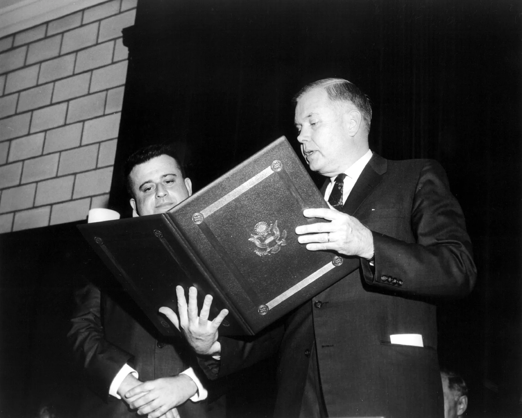
He was 26 when the paper appeared, and already fast. Born in Albany, New York, in 1927, he served in the Navy from 1944 to 1946, graduated from Harvard at 19 and took his doctorate at Chicago at 22, with Teller as his adviser. At Stanford in 1950 he worked out how electrons scatter off protons, a result still called the Rosenbluth formula. At Los Alamos, where he worked from 1950 to 1956, he spent his first years on the hydrogen bomb and, in Freeman Dyson’s words, made major contributions to the design of the first one, exploded in the Mike test of 1952. In 1954 he watched the Bravo test from a ship thirty or forty miles away, took ten rad of radiation, and remembered the fireball as “a diseased brain up in the sky”.
Then he turned to fusion, the same fire held still. In 1956 he left Los Alamos for General Atomic, and in 1957, with MacDonald and Judd, he published the Fokker–Planck equation for particles that act on each other through an inverse-square force, like the electric force between the charges of a plasma. Its two coefficients, the drift of a particle’s velocity and the spread of it, are written through two integrals of the distribution itself, still called the Rosenbluth potentials. The walk he and Arianna built becomes, in the limit, a diffusion governed by a Fokker–Planck equation; four years after it, he wrote the Fokker–Planck equation that plasma physicists use for collisions.
He worked at San Diego, at the Institute for Advanced Study and at Texas, where he was the founding director of the Institute for Fusion Studies, and from 1993 to 1998 he was chief scientist of ITER’s joint central team. He was often called the pope of plasma physics. Dyson, who knew both, wrote that “Enrico Fermi was the only other physicist I have known who was equal to Rosenbluth in his intuitive grasp of physics.” The National Medal of Science he received in 1997 cites “his fundamental contributions to plasma physics, his pioneering work in computational statistical mechanics”, the second being the work this post is about. Asked about renaming the algorithm, he answered that “life has been good to me”, and that he felt “rewarded in knowing that this algorithm will allow scientists to solve problems ranging from fluid flow to social dynamics to elucidating the nature of elementary particles.” He died of pancreatic cancer on 28 September 2003, three and a half months after the conference.
Arianna Wright was born in Houston in 1927 and earned her doctorate in physics at Harvard in 1949, at 21. She married Marshall in 1951; they had four children and divorced in 1978. After Los Alamos she did not work professionally again; she raised her children. She died on 28 December 2020, at 93, of complications of Covid-19. The program that first said no was hers. The name on the method belongs to the man who provided the computer time.
Sources
- F. Smets and R. Wouters, “Shocks and frictions in US business cycles: a Bayesian DSGE approach”, American Economic Review 97 (2007) 586–606; the step size and the rejection rate are in footnote 6 of the working-paper version, ECB Working Paper 722 (2007).
- Dynare’s settings and users: the Dynare reference manual, options mh_jscale and mh_tune_jscale, and the page About Dynare, dynare.org.
- G. O. Roberts, A. Gelman and W. R. Gilks, “Weak convergence and optimal scaling of random walk Metropolis algorithms”, The Annals of Applied Probability 7 (1997) 110–120.
- N. Metropolis, A. W. Rosenbluth, M. N. Rosenbluth, A. H. Teller and E. Teller, “Equation of state calculations by fast computing machines”, The Journal of Chemical Physics 21 (1953) 1087–1092.
- A. Gelman, G. O. Roberts and W. R. Gilks, “Efficient Metropolis jumping rules”, in J. M. Bernardo, J. O. Berger, A. P. Dawid and A. F. M. Smith (eds.), Bayesian Statistics 5, Oxford University Press (1996) 599–608.
- The one-dimensional optimum of 0.44: A. Gelman, J. B. Carlin, H. S. Stern, D. B. Dunson, A. Vehtari and D. B. Rubin, Bayesian Data Analysis, 3rd edition, CRC Press (2013), §12.2.
- N. R. Faria et al., “The early spread and epidemic ignition of HIV-1 in human populations”, Science 346 (2014) 56–61.
- BEAST’s default target acceptance rate of 0.234: the source code of BEAST v1.8.0, SimpleMCMCOperator, github.com/beast-dev/beast-mcmc.
- Planck Collaboration, “Planck 2018 results. VI. Cosmological parameters”, Astronomy & Astrophysics 641 (2020) A6.
- A. Lewis and S. Bridle, “Cosmological parameters from CMB and other data: a Monte Carlo approach”, Physical Review D 66 (2002) 103511.
- A. Lewis, “Efficient sampling of fast and slow cosmological parameters”, Physical Review D 87 (2013) 103529.
- H. Haario, E. Saksman and J. Tamminen, “An adaptive Metropolis algorithm”, Bernoulli 7 (2001) 223–242.
- G. O. Roberts and J. S. Rosenthal, “Optimal scaling of discrete approximations to Langevin diffusions”, Journal of the Royal Statistical Society: Series B 60 (1998) 255–268.
- S. Duane, A. D. Kennedy, B. J. Pendleton and D. Roweth, “Hybrid Monte Carlo”, Physics Letters B 195 (1987) 216–222.
- A. Beskos, N. Pillai, G. Roberts, J.-M. Sanz-Serna and A. Stuart, “Optimal tuning of the hybrid Monte Carlo algorithm”, Bernoulli 19 (2013) 1501–1534.
- J. E. Gubernatis, “Marshall Rosenbluth and the Metropolis algorithm”, Physics of Plasmas 12 (2005) 057303.
- M. N. Rosenbluth, “Genesis of the Monte Carlo algorithm for statistical mechanics”, AIP Conference Proceedings 690 (2003) 22–30.
- The 1964 E. O. Lawrence Award to Marshall N. Rosenbluth and its citation: U.S. Department of Energy, Office of Science, science.osti.gov/lawrence.
- P. H. Diamond, M. L. Goldberger, R. Z. Sagdeev and H. L. Berk, “Marshall Nicholas Rosenbluth”, Physics Today 57 (11) (2004) 82.
- His years at Harvard, in the Navy and at Texas: the memorial resolution for Marshall N. Rosenbluth of the University of Texas at Austin, by Berk, Mark and Weinberg.
- M. N. Rosenbluth, “High energy elastic scattering of electrons on protons”, Physical Review 79 (1950) 615–619.
- F. J. Dyson, “Marshall N. Rosenbluth”, Proceedings of the American Philosophical Society 150 (2006).
- M. N. Rosenbluth, interviewed by R. Rhodes on 26 May 1994, Voices of the Manhattan Project, Atomic Heritage Foundation.
- M. N. Rosenbluth, W. M. MacDonald and D. L. Judd, “Fokker–Planck equation for an inverse-square force”, Physical Review 107 (1957) 1–6.
- The 1997 National Medal of Science to Marshall N. Rosenbluth and its citation: nationalmedals.org.
- Arianna Rosenbluth’s marriage: S. Chen, APS News, 1 March 2022, on Arianna Rosenbluth and the Metropolis algorithm.
- K. Hafner, “Arianna Rosenbluth dies at 93; pioneering figure in data science”, The New York Times, 9 February 2021.
Every number in the text, the charts and the board are computed by the scripts archived with this post: random walks on Gaussian and flatter-topped targets in up to 500 dimensions, 30,000 walks on a 36-parameter posterior with a known answer, Langevin walks in 10,000 dimensions and a walk that tunes itself, all simulated once and saved.
Interested in applying these ideas to your work? Get in touch.