The Barrier That Comes Early

Two People, One Question

A contractor signs a one-year fixed-price job. Its copper comes from a supplier whose agreement has a clause: if the copper index, at 100 today, ever touches 120 before the job is finished, the supplier may reprice, and the contractor’s bid does not survive a repricing. Across town, a trader sells a one-year call on a stock at $100 with a knock-out clause: if the stock ever touches $120 before expiry, the option dies and pays nothing. It is called an up-and-out call.

They are asking the same question. What is the chance the price touches 120 before the year is out, and when is it most likely to happen?

Suppose copper grows about 4% a year on average, with a volatility of 20%. At that pace, it turns out, the average wait before the index first reaches 120 is 9.1 years. The contractor relaxes.

The contractor should not. The chance that the index touches 120 within the year is 39.6%, and the single most likely moment for it to happen is about three months from now.

The Convenience of a Logarithm

Both numbers come from one assumption, the one behind the Black–Scholes formula: the price follows a geometric Brownian motion, growing at a rate $\mu$ with volatility $\sigma$, its percentage moves independent from one moment to the next. Take its logarithm and the price becomes the simplest random process there is, a Brownian motion with a steady drift:

$$\ln S_t = \ln S_0 + \nu\,t + \sigma W_t, \qquad \nu = \mu – \tfrac{1}{2}\sigma^2$$

$(1)$

The barrier becomes a fixed distance away, $d = \ln(120/100) = 0.182$, and the drift of the logarithm is $\nu = 4\% – 2\% = 2\%$ a year. The question is now how long a drifting Brownian motion takes to walk a distance $d$, and that question has an exact answer. The time $\tau$ of the first touch has the density

$$f(t) = \frac{d}{\sigma\sqrt{2\pi t^3}}\,\exp\!\Big(-\frac{(d – \nu t)^2}{2\sigma^2 t}\Big)$$

$(2)$

and the chance that the touch has happened by a time $T$ is

$$P(\tau \le T) = \Phi\Big(\frac{\nu T – d}{\sigma\sqrt T}\Big) + e^{2\nu d/\sigma^2}\,\Phi\Big(\frac{-d – \nu T}{\sigma\sqrt T}\Big)$$

$(3)$

where $\Phi$ is the normal distribution function in every spreadsheet. With no drift, the formula collapses to twice the chance of ending the horizon above the barrier: a path that ends above 120 must have crossed it, and for every such path there is a mirror image that crossed and came back down. Louis Bachelier used exactly this reflection in his thesis on the Paris bourse in 1900.

That is the whole convenience. No simulation, no grid, no special function: three numbers, $d$, $\nu$ and $\sigma$, go into a formula a spreadsheet can hold, and out comes the full distribution of the waiting time.

Algorithm — The Chance of Crossing a Barrier

input:  S0   the price today
        B    the barrier, above S0
        σ    the yearly volatility
        μ    yearly growth (to plan), or r − q (to price)
        T    the horizon, in years

d  <- ln(B / S0)                  how far, in log terms
ν  <- μ − σ²/2                    the drift of the log price

P(crossed by T) <- Φ((νT − d)/(σ√T))
                   + exp(2νd/σ²) · Φ((−d − νT)/(σ√T))
P(ever crossed) <- 1 if ν ≥ 0, otherwise exp(2νd/σ²)
most likely time <- 2d² / (3σ² + √(9σ⁴ + 4ν²d²))
average time     <- d / ν         (only when ν > 0)

Nine Years, or Three Months?

Here is the distribution for the contractor’s copper, or the trader’s stock: $100 today, a barrier at $120, 20% volatility and 4% growth.

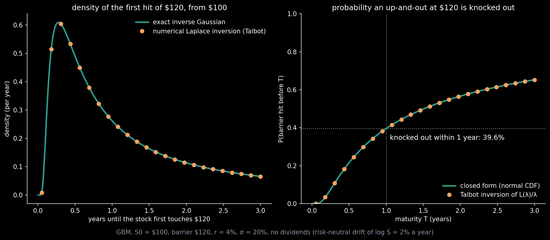
Left: the density of the time at which a price starting at $100 first touches $120, with 20% volatility and 4% growth. It peaks at about three months and then falls away slowly for years. Right: the chance that the touch has happened by each horizon; 39.6% within one year. The lines are the exact… — **Figure 1.** Left: the density of the time at which a price starting at $100 first touches $120, with 20% volatility and 4% growth. It peaks at about three months and then falls away slowly for years. Right: the chance that the touch has happened by each horizon; 39.6% within one year. The lines are the exact inverse Gaussian, and the dots the same curves recovered by numerically inverting its Laplace transform.

The chance of a touch is 7.5% within three months, 21.6% within six, 39.6% within a year, 56.7% within two and 74.4% within five. The most likely moment is 3.3 months away, the median a year and a half, and the average 9.1 years.

The average is not wrong; it is useless for planning. A drift of 2% a year against 20% noise means that most paths reach 120 fairly soon, while the unlucky ones wander downwards first and take decades to come back, and those few very long waits drag the average out to nine years. The density has a sharp early peak and an enormously long tail. Anyone who plans around the average waiting time of a first touch will be surprised early.

One Recipe for Every Process

The dots in Figure 1 were not drawn from the formula. They come from a recipe that works for any price that moves continuously, and it shows exactly where the convenience of GBM comes from.

For any such process, the Laplace transform of the hitting time, the average of $e^{-\lambda\tau}$, is a ratio of two values of one function:

$$\mathbb{E}\big[e^{-\lambda\tau}\big] = \frac{\psi_\lambda(S_0)}{\psi_\lambda(B)}, \qquad \tfrac12\,\sigma(S)^2\,\psi_\lambda^{\prime\prime} + \mu(S)\,\psi_\lambda^{\prime} = \lambda\,\psi_\lambda$$

$(5)$

where $\psi_\lambda$ is the increasing solution of the equation on the right, built from the process’s own drift and volatility. For GBM the equation is $\tfrac12\sigma^2S^2\psi^{\prime\prime} + \mu S\psi^{\prime} = \lambda\psi$, whose solutions are plain powers $S^\gamma$, so the ratio is elementary:

$$\mathbb{E}\big[e^{-\lambda\tau}\big] = \exp\Big(\frac{d\,\big(\nu – \sqrt{\nu^2 + 2\lambda\sigma^2}\big)}{\sigma^2}\Big)$$

$(6)$

Turning a transform back into a density is a numerical routine. The dots in Figure 1 are this one inverted by Talbot’s method, in the fixed form of Abate and Valkó: the inversion integral is bent into a contour that curls around the negative real axis, where the transform’s singularities lie, and sampled at seventy points. With the inputs given to 30 digits, it agrees with the inverse Gaussian to 30 significant digits. This is the whole method:

Algorithm — Talbot’s Inversion, Fixed Version

input:  F(λ)   the Laplace transform (Eq. 6 here, Eq. 7 below)
        t      the time at which the density is wanted
        M      the number of terms (70 for 30 digits)

r      <- 2M / 5
p0     <- r / t
term0  <- ½ · exp(r) · F(p0)
for k = 1 … M − 1:
    θ      <- kπ / M
    pk     <- (r / t) · θ · (cot θ + i)   on the contour
    termk  <- exp(t · pk) · F(pk) · (1 + iθ(1 + cot²θ) − i cot θ)
f(t)   <- (r / (M t)) · Re(term0 + term1 + … + termM−1)

work at about 1.7 times the digits wanted (51 for 30):
the terms far along the contour are huge and cancel

Now make the price mean-reverting, as a spread between two related prices or an interest rate is often modelled: the Ornstein–Uhlenbeck process, $dX = \theta(m – X)\,dt + \sigma\,dW$. The recipe is unchanged, but the equation is now Weber’s, and $\psi_\lambda$ is no longer a power. It is the parabolic cylinder function $D_\nu$. In units where $\theta = 1$, $\sigma = \sqrt2$ and $m = 0$, a level $b$ above the start $x$ is first reached with

$$\mathbb{E}\big[e^{-\lambda\tau}\big] = e^{(x^2 – b^2)/4}\,\frac{D_{-\lambda}(-x)}{D_{-\lambda}(-b)}$$

$(7)$

a formula that goes back to Darling and Siegert in 1953. No elementary density stands behind it, except for the one level the process keeps returning to, its own mean. So the numerical inversion is the working route, and it is the same Talbot inversion: from $x = -1$ up to the mean, it matches that one exact density to 30 significant digits as well.

That is the parallel. GBM’s convenience is that its special function happens to be elementary, a power. Mean reversion swaps the power for the parabolic cylinder function; a square-root process, like the ones behind many interest-rate and volatility models, swaps it for the confluent hypergeometric functions; a process confined to a range, for Gauss’s hypergeometric function. The recipe and the inversion carry over untouched.

Two Maps

Vary the barrier and the volatility, and the formula draws two maps. On the left, the density of the hitting time, for barriers from $105 to $160, at 20% volatility: a near barrier gives a tall, early peak, a far one a low, broad, late one. The teal line is the most likely moment, which grows roughly with the square of the distance; the orange dashes are the median. On the right, the chance of a knock-out within one year, over barrier and volatility.

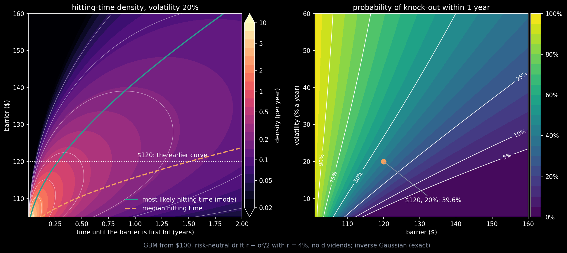
Left: the hitting-time density over time and barrier at 20% volatility, on a logarithmic colour scale, with the most likely hitting time (teal) and the median (orange); the dotted line is the $120 barrier of the previous figure. Right: the chance of a knock-out within one year over barrier and… — **Figure 2.** Left: the hitting-time density over time and barrier at 20% volatility, on a logarithmic colour scale, with the most likely hitting time (teal) and the median (orange); the dotted line is the $120 barrier of the previous figure. Right: the chance of a knock-out within one year over barrier and volatility; the dot is $120 at 20%, 39.6%.

The contours on the right are almost straight lines fanning out from $100. That is the formula talking: the chance depends mostly on one number, the distance to the barrier measured in standard deviations over the horizon, $d/(\sigma\sqrt T)$, so doubling the volatility has about the same effect as doubling the distance’s logarithm. The drift bends the lines. At 10% volatility the exact chance at $120 is 12.4%, against 6.8% if the drift is ignored, because 4% of growth pushes a calm price towards the barrier. At 40% volatility it is 61.9% against 64.9%: the $\sigma^2/2$ in $\nu$ has turned the drift of the logarithm negative, and it pulls the price away.

Read along a contour and you trade distance for volatility at a fixed risk. At 20% volatility, a barrier with a 10% chance of being touched within a year sits at $141; one with even odds sits at $115.70. At $120, even odds need 26.7% volatility.

The Board

Here are the same two maps, live. Every slider recomputes both from the exact formula as you drag it; hovering shows the value under the cursor, and the line under the top sliders prices the contract marked by the dot.

Two maps of the exact inverse Gaussian for a price starting at $100. Map 1 is the density of the hitting time over time and barrier; map 2 is the chance of a knock-out before maturity over barrier and volatility. The sliders set the interest rate (or growth) r, the dividend yield q, the contract's barrier, the volatility, the time window and the maturity; the dot on map 2 is the contract, and the summary line gives its knock-out chance, the most likely and the median hitting time, and the chance of ever touching the barrier.

For a contract, set r to the interest rate and q to the dividend yield: the board then shows the probabilities under which options are priced. For a project, read r − q as the growth you expect of the price, and the same maps become planning tools. Three things to try. Drag the maturity and watch the fan of contours sweep across map 2. Push the volatility past 30% with r at 4%, and watch the chance of ever touching the barrier fall below 100%. Then set r to zero.

Volatility Decides When, Not Whether

Setting r to zero shows the second surprise. If the price has no drift at all, a fair game, the chance that it ever reaches $120 from $100 is exactly 100/120, or 83.3%, whatever the volatility. More volatility only brings the moment forward: the chance of a touch within a year is 6.2% at 10% volatility, 33.0% at 20%, 58.9% at 40% and 73.9% at 80%, and the chance of a touch at all stays 83.3% throughout.

With growth the rule becomes

$$P(\text{the price ever reaches } B) = \min\Big(1,\ \big(S_0 / B\big)^{\,1 – 2\mu/\sigma^2}\Big)$$

$(4)$

and at 4% growth it produces a genuine reversal. Once the volatility passes $\sqrt{2\mu}$, 28.3%, more volatility makes a touch within the year more likely and a touch ever less likely: at 30% volatility the chance within a year is 53.8% and the chance ever 98.0%; at 50%, 67.0% and 88.3%; at 80%, 74.9% and 85.3%. A wild price reaches the barrier sooner if it reaches it at all, but more of its paths collapse and never come back.

What a Knock-Out Is Worth

The trader’s question has a price. A plain one-year call struck at $100, with 20% volatility and 4% interest, is worth $9.93. The up-and-out call with a barrier at $120 is worth $1.17, about an eighth. The knock-out removes more than its 39.6% suggests, because the paths that would have paid the most are exactly the ones that ran up through $120 on their way. What survives can pay at most $20.

Robert Merton gave the first price for a barrier option, a down-and-out call, in 1973, and the key is the reflection again: the joint law of the price and the highest level it has reached gives the up-and-out price as one integral. The integral gives $1.1671; a million simulated paths give $1.164, with a standard error of $0.003. The density prices anything paid at the moment of the touch too: $1 paid when the barrier is hit, if that happens within the year, is worth $0.388 today.

One practical correction. Most contracts check the barrier at the daily close, not continuously, and a price can cross $120 during the day and be back below by the close. Broadie, Glasserman and Kou showed that a daily barrier behaves like a continuous one moved outward by the factor $e^{0.5826\,\sigma\sqrt{\Delta t}}$, here from $120 to $120.88. With it, the chance of a knock-out falls from 39.6% to 37.6% (a million daily-checked paths give 37.62%) and the up-and-out price rises from $1.17 to $1.32, 13% more.

What the Formula Assumes

The convenience has a price of its own. The formula assumes a constant volatility, and markets do not keep one. It assumes the price moves continuously, while real prices gap overnight and on news, and a gap can jump straight through a barrier that a continuous path would have touched first. And the drift matters: to price a contract one uses the interest rate, as every trader must, but to plan a project one needs the growth one actually expects, which is harder to know than a volatility. The board is a first answer, fast and exact under its assumptions; it is the benchmark a more realistic model has to beat.

A Particle Falling Between Two Marks

The curve on the board was first written down in 1915, by two physicists at once. Erwin Schrödinger, eleven years before his wave equation, and Marian Smoluchowski were both thinking about the experiments of Robert Millikan and Felix Ehrenhaft, who measured the electric charge on tiny particles by timing them as they fell between two marks. Brownian motion made those falls irregular, and both men asked how long a particle jostled by molecules takes to cross a fixed distance. The answer was this density. Thirty years later Maurice Tweedie gave it its name, the inverse Gaussian, because it answers the inverse of the Gaussian’s question: the time needed to cover a fixed distance, where the Gaussian gives the distance covered in a fixed time.

The particle timed between two marks, the contractor watching copper and the trader who sold the knock-out are asking one question, and under a geometric Brownian motion it has one exact answer: the barrier tends to come much sooner than the average says.

Sources

L. Bachelier, “Théorie de la spéculation”, Annales scientifiques de l’École Normale Supérieure 17 (1900) 21–86.
A. Talbot, “The accurate numerical inversion of Laplace transforms”, IMA Journal of Applied Mathematics 23 (1979) 97–120.
J. Abate and P. P. Valkó, “Multi-precision Laplace transform inversion”, International Journal for Numerical Methods in Engineering 60 (2004) 979–993.
D. A. Darling and A. J. F. Siegert, “The first passage problem for a continuous Markov process”, Annals of Mathematical Statistics 24 (1953) 624–639.
R. C. Merton, “Theory of rational option pricing”, Bell Journal of Economics and Management Science 4 (1973) 141–183.
M. Broadie, P. Glasserman and S. Kou, “A continuity correction for discrete barrier options”, Mathematical Finance 7 (1997) 325–349.
E. Schrödinger, “Zur Theorie der Fall- und Steigversuche an Teilchen mit Brownscher Bewegung”, Physikalische Zeitschrift 16 (1915) 289–295.
M. von Smoluchowski, “Notiz über die Berechnung der Brownschen Molekularbewegung bei der Ehrenhaft-Millikanschen Versuchsanordnung”, Physikalische Zeitschrift 16 (1915) 318–321.
M. C. K. Tweedie, “Inverse statistical variates”, Nature 155 (1945) 453.

Every number in the text, the two figures and the board are computed by the scripts archived with this post, from the exact formulas, with Monte Carlo checks of the up-and-out price and the daily barrier and a 30-digit check of both Laplace inversions.

Interested in applying these ideas to your work? Get in touch.