
The Barrier Your Monte Carlo Never Sees
A Barrier Crossed Between Two Time Steps
A barrier option pays off — or is knocked out — depending on whether the underlying ever touches a level $B$ over the life of the contract. The event is defined in continuous time: the barrier is breached if the price dips below $B$ at any instant. But a Monte Carlo simulation only ever looks at a finite grid of times. Between two grid points the price can plunge through the barrier and climb back, and the simulation, seeing only the endpoints, records nothing.
The result is a silent, one-sided error. Naive path monitoring under-counts crossings, so it over-prices a down-and-out call and under-prices a down-and-in. Worse, the error shrinks with the time step at the punishing rate $\sqrt{\Delta t}$ — halving $\Delta t$ removes only about 30% of the bias. This post measures that bias, then removes almost all of it at essentially zero cost with a Brownian-bridge correction.
A Model We Can Grade Exactly
Take geometric Brownian motion with a down-barrier $B$. Working in log-price $X_t = \log S_t$ turns the multiplicative process into a Brownian motion with constant drift and volatility:
$(1)$
The crucial consequence: the log-increments are exactly Gaussian, so we can simulate the marginal distribution of $X$ with no discretization error at all. Any bias we see is therefore purely a monitoring artifact — the barrier check, not the path, is what is wrong. And because $X$ is Brownian motion with drift, the true continuous probability of ever crossing the log-barrier $b = \log B$ has a closed form from the reflection principle:
$(2)$
This is the number every estimator below is trying to hit.
What Happens Between the Nodes: a Brownian Bridge
Here is the idea that fixes everything. Condition on two consecutive simulated values $X_n$ and $X_{n+1}$. Over the interval $[t_n, t_{n+1}]$ the process is not free — it is a Brownian bridge pinned at both ends. And the probability that a Brownian bridge dips below a level $b$ somewhere inside the interval, given that both endpoints sit above it, is known in closed form:
$(3)$
When either endpoint is already at or below $b$, the step has crossed for certain and $p_n = 1$. Notice the shape: if either endpoint hugs the barrier, $(X_n – b)$ or $(X_{n+1} – b)$ is small, $p_n$ is close to $1$, and the correction fires hard — exactly the near-misses the naive check throws away. Treat each step’s crossing as an independent conditional event and the survival probability is the product over steps, giving the corrected hit estimator:
$(4)$
No extra paths, no finer grid — one exponential per step, evaluated on data we already have.
Algorithm — Brownian-Bridge Barrier Correction
input: X0, drift nu, vol sigma, log-barrier b, horizon T, steps L, paths M
dt <- T / L
for each of M paths:
    simulate X_1..X_L by exact log-increments:  X_{n+1} = X_n + Normal(nu*dt, sigma^2 * dt)
    survive <- 1
    for n = 0 .. L-1:
        if X_n <= b or X_{n+1} <= b:
            p_n <- 1                                      # a node is already through
        else:
            p_n <- exp(-2 * (X_n - b) * (X_{n+1} - b) / (sigma^2 * dt))
        survive <- survive * (1 - p_n)
    hit <- 1 - survive
return  mean of hit over the M paths
The Experiment
Estimate the down-hit probability three ways at a range of monitoring frequencies: naive grid monitoring (check the nodes only), the Brownian-bridge correction, and the exact continuous value $p_\star$ as the reference.
Python 3.13 — Brownian-Bridge Barrier Correction for GBM
import numpy as np
import matplotlib
matplotlib.use("Agg")
import matplotlib.pyplot as plt
from math import erf, sqrt

Phi = lambda z: 0.5 * (1.0 + erf(z / sqrt(2.0)))

# GBM  dS = mu S dt + sigma S dW,  down-barrier B.  Log-price X = log S is exact BM.
S0, B, mu, sigma, T = 100.0, 90.0, 0.05, 0.30, 1.0
X0, b = np.log(S0), np.log(B)
nu = mu - 0.5 * sigma**2

# exact continuous down-hit probability (reflection principle)
a = b - X0
p_star = (Phi((a - nu*T)/(sigma*sqrt(T)))
          + np.exp(2*nu*a/sigma**2) * Phi((a + nu*T)/(sigma*sqrt(T))))

def mc_hit(L, M, rng):
    dt = T / L
    incr = rng.normal(nu*dt, sigma*np.sqrt(dt), size=(M, L))     # exact log-increments
    X = X0 + np.cumsum(incr, axis=1)
    Xprev = np.concatenate([np.full((M, 1), X0), X[:, :-1]], axis=1)
    naive = np.mean(np.min(X, axis=1) <= b)                      # grid nodes only
    both = (Xprev > b) & (X > b)
    p = np.where(both, np.exp(-2.0*(Xprev - b)*(X - b)/(sigma**2*dt)), 1.0)
    bridge = np.mean(1.0 - np.prod(1.0 - p, axis=1))             # bridge-corrected
    return naive, bridge

rng = np.random.default_rng(1)
Ls = np.array([2, 4, 8, 16, 32, 64, 128, 256])
naive_ps, bridge_ps = np.array([mc_hit(int(L), 60000, rng) for L in Ls]).T
slope = np.polyfit(np.log(T/Ls), np.log(p_star - naive_ps), 1)[0]

# one illustrative path (seed chosen so it dips below B between two grid nodes)
Nf, Lc = 2048, 8
dtf = T / Nf
xf = np.concatenate([[X0], X0 + np.cumsum(
    np.random.default_rng(662).normal(nu*dtf, sigma*np.sqrt(dtf), size=Nf))])
tf = np.linspace(0, T, Nf+1)
idx = np.linspace(0, Nf, Lc+1).astype(int)
S = np.exp(xf)

NAVY, TEAL, RED, GREY = "#1e3a5f", "#2a9d8f", "#c0392b", "#8a8f98"
fig, (axL, axR) = plt.subplots(1, 2, figsize=(12.5, 5.2), facecolor="white",
                               gridspec_kw={"width_ratios": [1.05, 1]})

lo = min(S.min(), B) - 3.0
axL.axhspan(lo, B, color=RED, alpha=0.06)
axL.axhline(B, color=RED, lw=1.4, ls="--")
axL.plot(tf, S, color=NAVY, lw=1.2, label="true continuous path")
axL.plot(tf[idx], S[idx], "o", color=NAVY, ms=8, mfc="white", mew=1.8,
         label="monitored grid nodes")
axL.fill_between(tf, S, B, where=S < B, color=RED, alpha=0.5, lw=0)
j = np.argmin(S)
axL.annotate("the crossing the\ngrid never sees", xy=(tf[j], S[j]),
             xytext=(tf[j]-0.32, lo+1.2), color=RED, fontsize=10.5, fontweight="bold",
             arrowprops=dict(arrowstyle="->", color=RED, lw=1.5))
axL.text(0.015, B+0.6, "barrier  B = 90", color=RED, fontsize=10, fontweight="bold")
axL.set_xlim(0, T); axL.set_ylim(lo, S.max()+2)
axL.set_xlabel("time  $t$"); axL.set_ylabel("asset price  $S_t$")
axL.set_title("Every node is above the barrier — yet the path crossed", fontsize=11.5)
axL.legend(loc="upper right", framealpha=0.85, fontsize=9.5)
axL.spines[["top", "right"]].set_visible(False)

axR.axhline(p_star, color=GREY, lw=1.6, ls="--",
            label=f"exact continuous  $p_\\star = {p_star:.3f}$")
axR.plot(Ls, naive_ps, "o-", color=NAVY, lw=1.7, ms=7,
         label=f"naive grid monitoring  (bias $\\sim\\Delta t^{{{slope:.2f}}}$)")
axR.plot(Ls, bridge_ps, "s-", color=TEAL, lw=1.7, ms=7,
         label="Brownian-bridge corrected")
axR.set_xscale("log", base=2); axR.set_xticks(Ls); axR.set_xticklabels(Ls)
axR.set_xlabel("monitoring steps  $L = T/\\Delta t$")
axR.set_ylabel("estimated barrier-hit probability")
axR.set_title("The naive estimator crawls up at rate $\\sqrt{\\Delta t}$", fontsize=11.5)
axR.set_ylim(0.40, 0.78)
axR.legend(loc="lower right", framealpha=0.85, fontsize=9.5)
axR.spines[["top", "right"]].set_visible(False)
axR.grid(True, axis="y", alpha=0.25)

fig.tight_layout(pad=1.4)
fig.savefig("fig_1.png", dpi=150, bbox_inches="tight")
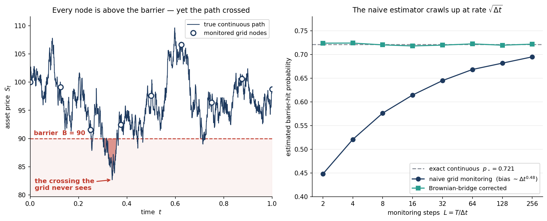
What the Plot Says
The two curves could not be more different. Naive monitoring starts at $0.45$ against a truth of $0.72$ — a 38% relative under-count — and even at $256$ steps it has only crawled up to $0.70$. The fitted convergence rate is $\Delta t^{0.48}$, right on the theoretical $\sqrt{\Delta t}$ of Broadie, Glasserman, and Kou. That half-order is brutal: to cut the bias by a factor of ten you need a hundred times as many steps.
The bridge-corrected estimator, by contrast, is flat on the exact line from $L = 2$ onward. This is not a coincidence of tuning. Because the log-increments are exact and the bridge-crossing probability in equation (3) is exact conditional on the endpoints, the estimator is unbiased for the continuous crossing probability at any step count — the only thing left is ordinary Monte Carlo noise, which the jitter in the teal curve makes visible. Two time steps recover what naive monitoring cannot reach with two hundred and fifty-six.
When It Matters, and What to Watch
The correction earns its keep exactly when the barrier is close to the money or the volatility is high — the regime where near-misses between nodes are common and the naive bias is largest. It generalises well beyond this toy: any scheme that gives you consecutive values of an approximately-Gaussian increment (Euler, Milstein, an exact scheme) can carry the same per-step bridge probability, and the trick extends to time-dependent and double barriers with the same conditioning argument.
Two honest caveats. The bridge formula assumes constant $\sigma$ within a step, so for a genuinely path-dependent diffusion you are approximating the local bridge — still far better than ignoring the excursion, but no longer exact. And under a discretization scheme that carries its own weak error, the bridge removes the monitoring bias but not the scheme bias; the two are separate defects and only the first is fixed here. Neither caveat dents the headline: the term the grid drops is the whole error, and one exponential per step buys it back.
Working on a pricing model or risk system? Let’s talk.