The 1/√N Wall: Why Monte Carlo Is Slow, and What Beats It

The Error That Refuses to Fall Fast

Monte Carlo is the workhorse of quantitative practice: to estimate an expectation, draw samples and average them. It is trivial to code, it copes with high dimension, and it comes with a guarantee of convergence. What it does not come with is speed. The estimate improves, but it improves slowly — and the slowness is not an implementation detail you can optimise away. It is baked into the statistics.

This post pins down exactly how slow, why, and what changes the exponent rather than just the constant.

Where the Square Root Comes From

Suppose we want $I = \mathbb{E}[f(U)]$ for $U$ uniform on the unit cube, and we estimate it with the sample mean of $N$ independent draws:

The estimator is unbiased, so all of the error is variance. Because the draws are independent, the variance of the average is the variance of one term divided by $N$:

The standard error is the square root of that:

There is the wall. The typical error decays like $N^{-1/2}$, and no amount of cleverness in the random number generator changes the exponent. To halve the error you must quadruple the sample count. To gain one more decimal digit you pay a factor of one hundred. This is why a Monte Carlo pricer that is accurate to a basis point can be genuinely expensive, and why variance — the size of $\sigma$ — matters far more than raw sample throughput.

The one lever the square-root law leaves you is $\sigma$: variance-reduction tricks (antithetics, control variates, importance sampling) shrink the constant in front of $N^{-1/2}$. They can be worth a large factor. But they leave the slope alone. To bend the slope, you have to attack the assumption that produced it — independence.

Randomness Is the Problem, Not the Solution

The $N^{-1/2}$ rate is a direct consequence of using independent random points. Independence is convenient for the variance algebra, but it is wasteful as a way to cover a space: random points clump. Purely by chance you get clusters here and gaps there, and those gaps are exactly the regions your average fails to see. The clumping is the error.

Quasi-Monte Carlo (QMC) abandons independence and instead lays down a deterministic low-discrepancy sequence — points engineered to fill the cube as evenly as possible at every scale. Discrepancy is a precise measure of how far a point set deviates from perfectly uniform coverage, and the Koksma–Hlawka inequality bounds the integration error by the product of the function’s variation and the point set’s discrepancy:

The good sequences — Halton, Sobol′, Faure — achieve star-discrepancy $D_N^{*} = O\!\big((\log N)^{d}/N\big)$. Ignore the logarithms and the rate is essentially $N^{-1}$, not $N^{-1/2}$. That is the whole game: the error falls roughly twice as fast on the log-log plot, so the same accuracy costs the square root of the sample count.

Measuring the Gap

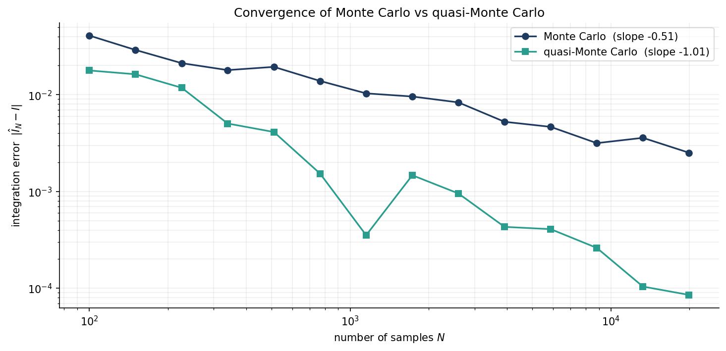
Talk is cheap; the exponent is measurable. We integrate a smooth test function over the unit square with both methods across a sweep of sample sizes, and fit the slope of error against $N$ on log axes. The QMC points are a Halton sequence in bases 2 and 3; the Monte Carlo error is averaged over repeated trials so we plot the typical error, not one lucky draw.

import numpy as np
import matplotlib
matplotlib.use("Agg")
import matplotlib.pyplot as plt

# integrate a smooth test function over the unit square; true value known
def f(x, y):
    return np.exp(-(x**2 + y**2)) * (1.0 + np.sin(3.0 * np.pi * x * y))

# reference value from a huge dense grid
g = np.linspace(0.5/4000, 1 - 0.5/4000, 4000)
X, Y = np.meshgrid(g, g)
I_true = f(X, Y).mean()

def halton(n, base):                       # deterministic low-discrepancy sequence
    v = np.zeros(n)
    for i in range(n):
        f_, r, k = 1.0, 0.0, i + 1
        while k > 0:
            f_ /= base
            r += f_ * (k % base)
            k //= base
        v[i] = r
    return v

rng = np.random.default_rng(0)
Ns = np.unique(np.round(np.logspace(2, 4.3, 14)).astype(int))
mc, qmc = [], []
for N in Ns:
    errs = []                              # plain MC: typical error over 30 trials
    for _ in range(30):
        p = rng.random((N, 2))
        errs.append(abs(f(p[:, 0], p[:, 1]).mean() - I_true))
    mc.append(np.mean(errs))
    hx, hy = halton(N, 2), halton(N, 3)    # QMC: single Halton point set
    qmc.append(abs(f(hx, hy).mean() - I_true))

mc, qmc = np.array(mc), np.array(qmc)
s_mc = np.polyfit(np.log(Ns), np.log(mc), 1)[0]
s_qmc = np.polyfit(np.log(Ns), np.log(qmc), 1)[0]

NAVY, TEAL = "#1e3a5f", "#2a9d8f"
fig, ax = plt.subplots(figsize=(10, 5), facecolor="white")
ax.loglog(Ns, mc, "o-", color=NAVY, lw=1.6, ms=6, label=f"Monte Carlo  (slope {s_mc:.2f})")
ax.loglog(Ns, qmc, "s-", color=TEAL, lw=1.6, ms=6, label=f"quasi-Monte Carlo  (slope {s_qmc:.2f})")
ax.set_xlabel(r"number of samples $N$")
ax.set_ylabel(r"integration error  $|\hat I_N - I|$")
ax.set_title("Convergence of Monte Carlo vs quasi-Monte Carlo")
ax.legend(framealpha=0.7)
ax.spines[["top", "right"]].set_visible(False)
ax.grid(True, which="both", alpha=0.2)
fig.tight_layout(pad=1.5)
fig.savefig("fig_1.png", dpi=150, bbox_inches="tight")

What the Slopes Say

The fitted slopes come out Monte Carlo $\approx -0.51$ and quasi-Monte Carlo $\approx -1.02$ — almost exactly the theoretical $-\tfrac{1}{2}$ and $-1$. This is not a constant-factor speedup; it is a different rate. At the right-hand edge of the plot the QMC error is more than an order of magnitude below MC, and the gap grows the further you push. Read the other way: to reach the accuracy QMC has at ten thousand points, plain Monte Carlo would need on the order of a million.

When It Wins, and When It Doesn’t

Quasi-Monte Carlo is not free lunch, and it is worth being honest about the fine print.

Smoothness matters. The Koksma–Hlawka bound carries the function’s total variation $V(f)$. For smooth, well-behaved integrands the QMC advantage is dramatic; for discontinuous payoffs — a digital option, a barrier — $V(f)$ blows up and the advantage erodes toward the Monte Carlo rate. Smoothing the integrand first is often what makes QMC pay.

Dimension matters, but less than the bound suggests. That $(\log N)^d$ factor looks fatal in high dimension, yet in practice QMC keeps winning on problems nominally in the hundreds of dimensions. The reason is effective dimension: many finance integrands are dominated by a few directions, and a Brownian-bridge or PCA construction loads the important variance onto the first, best-covered coordinates.

You lose the free error bar. A deterministic sequence gives you a number, not a confidence interval — the honest simplicity of the Monte Carlo standard error is gone. The fix is randomised QMC (scrambled Sobol′, shifted lattices): average over a handful of independent scrambles and you recover an unbiased estimate and a variance estimate, while keeping most of the fast rate.

The takeaway is blunt. If your simulation is smooth and you care about the last digit, the square-root wall is not a law of nature — it is a consequence of throwing points down at random. Stop doing that, cover the space deliberately, and the same accuracy costs the square root of the effort.

Need a reliable numerical implementation for your problem? Get in touch.