Euler–Maruyama vs Milstein: The Term That Matters

Discretizing a Stochastic Differential Equation

Most stochastic differential equations have no closed-form solution, so we simulate them on a grid. Given

$$dX_t = a(X_t)\,dt + b(X_t)\,dW_t,$$

$(1)$

we step forward in time with increments of the Brownian motion. But how well a scheme tracks the true path is not obvious, and the answer separates two classic methods by a full order of accuracy. This post measures that gap directly.

The right yardstick here is strong convergence — how close the numerical path stays to the exact path driven by the same Brownian motion:

$$e(\Delta t) = \mathbb{E}\,\big|X_T^{\Delta t} – X_T\big| \le C\,(\Delta t)^{\gamma}.$$

$(2)$

The exponent $\gamma$ is the strong order. Bigger is better: halving $\Delta t$ cuts the error by $2^{\gamma}$.

A Test Equation We Can Grade

Geometric Brownian motion, $a(x)=\lambda x$ and $b(x)=\mu x$, has an exact solution driven by the same path:

$$X_t = X_0 \exp\!\Big(\big(\lambda – \tfrac{1}{2}\mu^2\big)t + \mu W_t\Big).$$

$(3)$

So for any simulated path we can compute the true endpoint from $W_T$ and measure the error exactly — no reference discretization needed.

Euler–Maruyama: the Obvious Scheme

The direct analogue of the Euler method: freeze the coefficients over each step and add a Gaussian Brownian increment $\Delta W \sim \mathcal{N}(0, \Delta t)$.

Algorithm — Euler–Maruyama Step

input: X0, drift a(x), diffusion b(x), step Dt, number of steps L
X <- X0
for n = 1 .. L:
    draw  dW ~ Normal(0, Dt)
    X <- X + a(X)*Dt + b(X)*dW
return X

Simple and cheap — but its strong order is only $\gamma = \tfrac{1}{2}$. The culprit is the term it silently drops.

Milstein: One More Term, Twice the Order

The Itô–Taylor expansion of the increment carries a second-order piece that Euler ignores. Because $\Delta W^2$ has mean $\Delta t$ (not zero), that piece contributes at first order. Milstein’s scheme keeps it:

$$X_{n+1} = X_n + a(X_n)\,\Delta t + b(X_n)\,\Delta W + \tfrac{1}{2}\,b(X_n)\,b'(X_n)\big(\Delta W^2 – \Delta t\big).$$

$(4)$

Algorithm — Milstein Step

input: X0, a(x), b(x), b'(x), step Dt, number of steps L
X <- X0
for n = 1 .. L:
    draw  dW ~ Normal(0, Dt)
    X <- X + a(X)*Dt + b(X)*dW + 0.5*b(X)*b_prime(X)*(dW*dW - Dt)
return X

The price is one extra term and the requirement that you know the derivative $b'(x)$ of the diffusion — for GBM, $b(x)=\mu x$ so $b'(x)=\mu$. The payoff is strong order $\gamma = 1$.

The Experiment

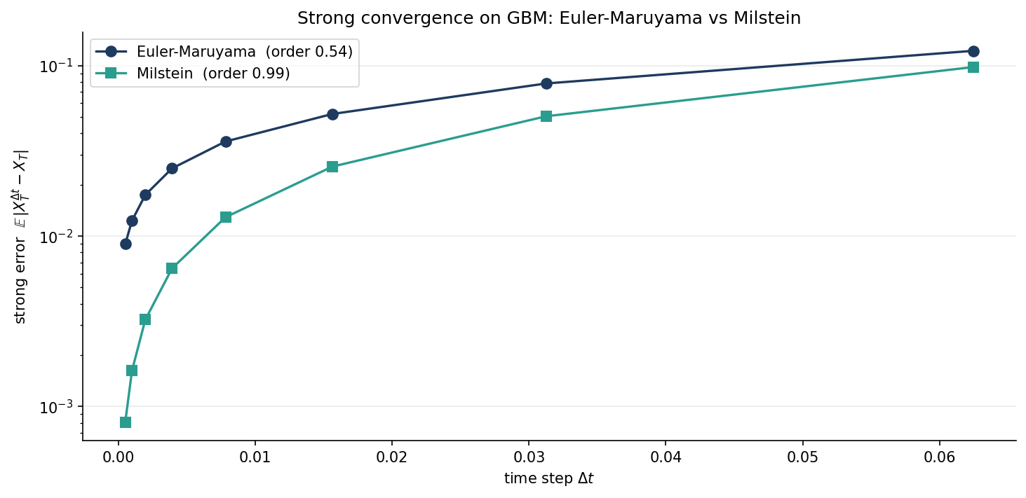
Simulate both schemes on the same Brownian paths at a range of step sizes, and measure the strong error against the exact solution:

Python 3.13 — Strong Convergence of Euler–Maruyama and Milstein

import numpy as np
import matplotlib
matplotlib.use("Agg")
import matplotlib.pyplot as plt

rng = np.random.default_rng(1)
lam, mu, X0, T = 1.0, 0.5, 1.0, 1.0        # dX = lam*X dt + mu*X dW  (GBM)
N = 2**12; dt = T/N; M = 2000              # fine grid, M paths

dW = rng.normal(0.0, np.sqrt(dt), size=(M, N))
Xtrue = X0*np.exp((lam - 0.5*mu**2)*T + mu*dW.sum(axis=1))   # exact endpoint

def strong_err(scheme, R):                 # R = coarsening factor
    L = N // R; Dt = R*dt
    dWc = dW[:, :L*R].reshape(M, L, R).sum(axis=2)           # coarse increments
    X = np.full(M, float(X0))
    for j in range(L):
        dWj = dWc[:, j]
        if scheme == "euler":
            X = X + lam*X*Dt + mu*X*dWj
        else:                              # milstein: b=mu*X, b'=mu
            X = X + lam*X*Dt + mu*X*dWj + 0.5*mu**2*X*(dWj**2 - Dt)
    return Dt, np.mean(np.abs(X - Xtrue))

dts, ee, me = [], [], []
for R in [2**p for p in range(1, 9)]:
    Dt, e = strong_err("euler", R);    dts.append(Dt); ee.append(e)
    _,  m = strong_err("milstein", R); me.append(m)

se = np.polyfit(np.log(dts), np.log(ee), 1)[0]      # measured slopes
sm = np.polyfit(np.log(dts), np.log(me), 1)[0]

NAVY, TEAL = "#1e3a5f", "#2a9d8f"
fig, ax = plt.subplots(figsize=(10, 5), facecolor="white")
ax.semilogy(dts, ee, "o-", color=NAVY, lw=1.6, ms=7, label=f"Euler-Maruyama  (order {se:.2f})")
ax.semilogy(dts, me, "s-", color=TEAL, lw=1.6, ms=7, label=f"Milstein  (order {sm:.2f})")
ax.set_xlabel(r"time step $\Delta t$")
ax.set_ylabel(r"strong error  $\mathbb{E}\,|X_T^{\Delta t} - X_T|$")
ax.set_title("Strong convergence on GBM: Euler-Maruyama vs Milstein")
ax.legend(framealpha=0.7)
ax.spines[["top", "right"]].set_visible(False)
ax.grid(True, which="major", axis="y", alpha=0.25)
fig.tight_layout(pad=1.5)
fig.savefig("fig_1.png", dpi=150, bbox_inches="tight")

**Figure 1.** Strong error against the exact solution versus step size $\Delta t$ (log scale on the error axis). As the grid refines, Milstein (teal) falls away far faster than Euler–Maruyama (navy) — the fitted convergence orders are $1/2$ and $1$.

What the Slopes Say

The fitted slopes come out Euler $\approx 0.54$ and Milstein $\approx 0.99$ — right on the theoretical $\tfrac{1}{2}$ and $1$. That is not a cosmetic difference: at $\Delta t = 10^{-3}$ the Milstein error is already an order of magnitude smaller, and the gap widens as the grid refines. One extra term, evaluated at no meaningful extra cost, buys a full order of strong accuracy.

When Each One Wins

Milstein is the clear choice for a scalar SDE whenever you can write down $b'(x)$ — which is most of the time. Euler–Maruyama keeps its place for two honest reasons: it needs no derivative of the diffusion, and in the multidimensional case Milstein’s correction involves iterated Itô integrals (Lévy areas) that are awkward to simulate, so the simple scheme is often what survives contact with a real model. And if you only care about weak convergence — expectations of payoffs rather than pathwise accuracy — both schemes are order one, and the picture changes again. But for tracking a path, the lesson of the plot is blunt: the term Euler drops is the term that matters.

Need a reliable numerical implementation for your problem? Get in touch.