The Rule That Fits One Ward

The Number on the Wall

Ask a hospital manager how full the beds should be and the answer often comes back as one number: 85%. Keep average occupancy at or below it, and a bed will almost always be free when an emergency arrives. The number traces back to a 1999 simulation study in the BMJ by Bagust, Place and Posnett, who found that the risk of an emergency patient finding no bed rises substantially once average occupancy passes 85%. It has been repeated in plans and reports ever since, usually as if it held for any hospital.

**Figure 1.** A ward at night. A painting.

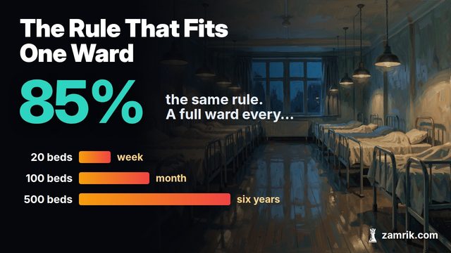
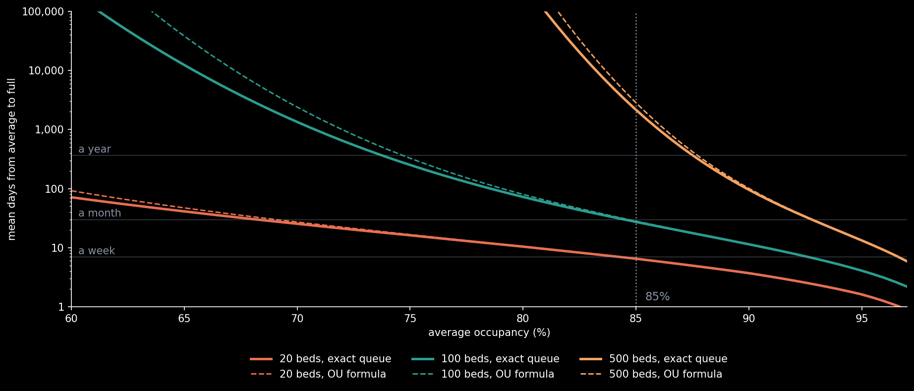
Take a ward of 100 beds run at 85%, with patients staying five days on average. How often is it completely full? About once a month: starting from its average of 85 occupied beds, it takes 27 days on average to reach 100. Now keep the same 85% and change only the size. A ward of 20 beds is full within 6.5 days. A hospital of 500 beds waits almost six years.

Same rule, three hospitals, and the waits differ by a factor of three hundred.

Beds That Come and Go

Patients arrive at random, $a$ of them a day on average, and each stays for a random time with mean $L$ days. The number of occupied beds is then the infinite-server queue, and for a ward of any real size it behaves like an Ornstein–Uhlenbeck process, as Donald Iglehart showed in 1965:

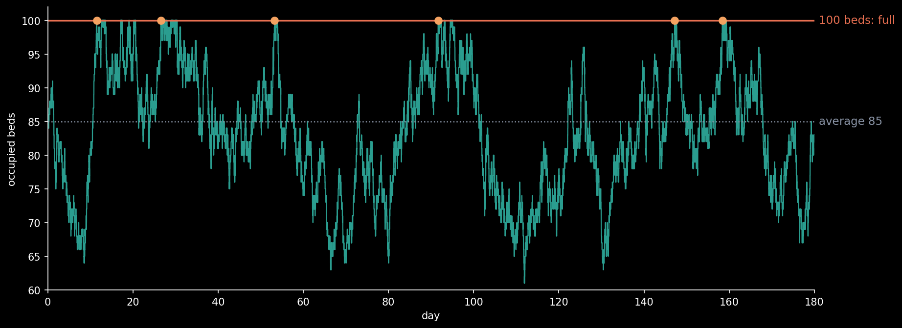
$$dX_t = \kappa\,(\theta – X_t)\,dt + \sigma\,dW_t, \qquad \kappa = \frac{1}{L}, \quad \theta = aL, \quad \sigma = \sqrt{2a}$$

$(1)$

Each parameter is something a ward already knows. $\theta$ is the average occupancy. $\kappa$, one over the length of stay, is how fast the ward forgets a busy day. $\sigma$ is the noise of admissions. Left alone, occupancy settles into a bell curve around $\theta$ with a standard deviation of $\sqrt{\theta}$, so a ward that averages 85 patients spends about two days in three between 76 and 94.

**Figure 2.** Six simulated months of a 100-bed ward at an average of 85%, stays of five days, patient by patient. A patient who arrives at a full ward goes elsewhere. Each dot is the first time the ward is full after coming back down to its average: six in this run, 5.7 in an average half-year.

How Long Until Full

The question is a first hitting time: how long until $X$ first reaches $c$, the number of beds. For the Ornstein–Uhlenbeck process it has an exact answer, because the process has an exact resolvent, the operator that turns a function of the state into its discounted future:

$$\begin{aligned} (R_\lambda f)(x) &= \mathbb{E}_x\!\int_0^\infty e^{-\lambda t} f(X_t)\,dt = \int G_\lambda(x,y)\,f(y)\,dy, \\ G_\lambda(x,y) &= \frac{\Gamma(\lambda/\kappa)}{\sigma\sqrt{\pi\kappa}}\; e^{(z_x^2 – z_y^2)/4}\, D_{-\lambda/\kappa}(-z_{x\wedge y})\, D_{-\lambda/\kappa}(z_{x\vee y}) \end{aligned}$$

$(2)$

Here $z = (x-\theta)\sqrt{2\kappa}/\sigma$ counts the occupancy in standard deviations from its average, which for a ward is $(x-\theta)/\sqrt{\theta}$, and $D_\nu$ is Weber’s parabolic cylinder function. From the resolvent comes the law of the first time $T_c$ the ward is full, through its Laplace transform (Darling and Siegert, 1953):

$$\mathbb{E}_x\big[e^{-\lambda T_c}\big] = e^{(z_x^2-\beta^2)/4}\,\frac{D_{-\lambda/\kappa}(-z_x)}{D_{-\lambda/\kappa}(-\beta)}, \qquad \beta = \frac{c-\theta}{\sqrt{\theta}}$$

$(3)$

and, differentiating at $\lambda = 0$, the mean wait:

$$\mathbb{E}_x[T_c] = \frac{1}{\kappa}\int_{z_x}^{\beta}\sqrt{2\pi}\,\Phi(u)\,e^{u^2/2}\,du$$

$(4)$

Everything that size, occupancy and length of stay do is carried by one number, $\beta$: how many standard deviations separate the average from a full ward. For 100 beds at 85%, $\beta = 1.63$, and the formula gives 28.2 days. The exact queue, counted patient by patient, gives 27.3.

Algorithm — Days Until the Ward Is Full

input:  c   number of beds
        θ   average occupied beds
        L   average stay, in days
β ← (c − θ) / √θ              distance to full, in sds
I ← ∫₀^β √(2π) Φ(u) exp(u²/2) du   by quadrature
days ← L · I                  mean wait from the average
ν₁ ← first zero of ν ↦ D_ν(−β)   bisection in log ν
P(no fill in t days) ≈ exp(−ν₁ t / L)
return days, ν₁

Same 85%, Three Hospitals

At a fixed occupancy $\rho$, the distance is $\beta = (1-\rho)\sqrt{c/\rho}$, and it grows with the square root of the number of beds. At 85%, a 20-bed ward sits 0.73 standard deviations from full, a 100-bed ward 1.63 and a 500-bed hospital 3.64. The wait grows faster than exponentially in $\beta$, so the same percentage means a week for the first, a month for the second and six years for the third.

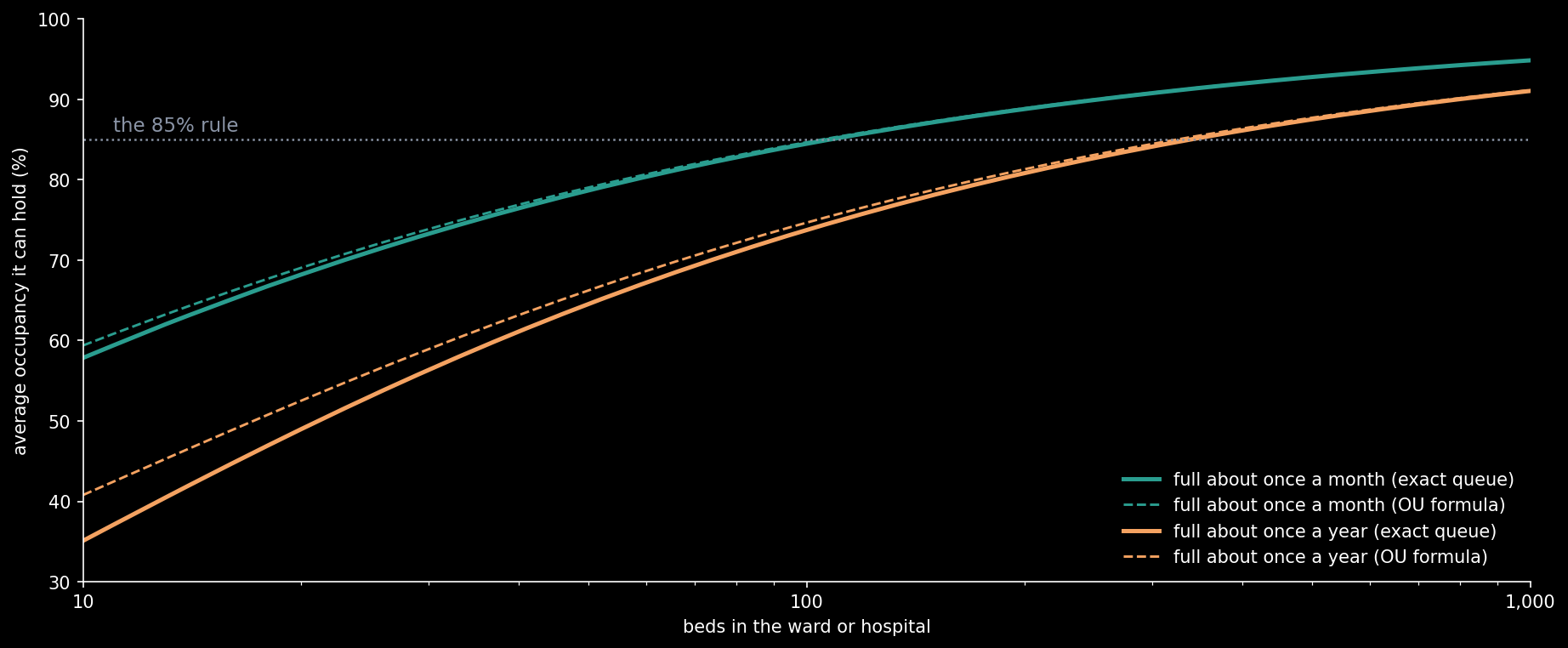
**Figure 3.** The mean wait from average occupancy to a full ward, against the average occupancy, for 20, 100 and 500 beds and stays of five days. Solid: the exact queue. Dashed: the Ornstein–Uhlenbeck formula. The dotted line is 85%.

Turn it round and ask which average occupancy keeps a ward about a month away from full. For 100 beds it is 84.5%. So the 85% rule is right for exactly one ward: one of about a hundred beds whose managers accept being full once a month. For 20 beds the same standard is 68%, and for 500 beds, 93%. To be full only about once a year, 20 beds must run at 49%, 100 beds at 74% and 500 beds at 88%.

A ward’s reserve is not a percentage but a number of standard deviations. Its spare beds should grow with the square root of its average: the square-root rule that Halfin and Whitt put on a firm footing for queues with many servers, and by which call centres now staff their lines.

**Figure 4.** The average occupancy a ward or hospital can hold, against its size, if it is to be full about once a month (teal) or once a year (orange). Solid: the exact queue. Dashed: the Ornstein–Uhlenbeck formula. Stays of five days.

A Full Ward Is Never Due

The transform holds one more surprise. It has poles at $\lambda = -\kappa\nu_n$, where $\nu_1 < \nu_2 < \dots$ are the zeros of $\nu \mapsto D_\nu(-\beta)$, so the chance of still waiting at time $t$ is a sum of decaying exponentials $e^{-\kappa\nu_n t}$ (Linetsky, 2004; Alili, Patie and Pedersen, 2005). The first pole sets how often a settled ward fills; the others only decide how fast it settles. For 100 beds at 85% the first pole gives one fill every 28.7 days, and the slowest eigenvalue of the exact queue gives 28.0.

Because one pole dominates, the wait is nearly exponential, and an exponential clock has no memory. A 100-bed ward at 85% has about a one-in-three chance, 34%, of getting through a month without filling up. A ward that has just done so has the same one-in-three chance for the next month. The full ward is never “due”.

The transform itself needs no inversion to be useful. If some other event arrives at random at rate $\lambda$, a surge of flu for instance, then $\mathbb{E}[e^{-\lambda T_c}]$ is exactly the chance that the ward is full before it comes. If surges come every 60 days on average, a 100-bed ward at 85% fills first with probability 68% by the formula, and 69% for the exact queue.

What the Model Leaves Out

Real admissions are not a steady random stream: they peak early in the week and in winter, and a ward that is fuller at the peaks is full more often. So these figures are a best case. The diffusion is accurate near full, within about 3% for waits of days and weeks, but it is optimistic for rare events: for 500 beds at 85% it says 7.8 years where the exact queue says 5.9, because real occupancy has a longer upper tail than the bell curve.

A Telephone Exchange in Copenhagen

This mathematics was not born in a hospital. In 1909 Agner Krarup Erlang, an engineer and mathematician at the Copenhagen Telephone Company, showed that calls arriving at random follow Poisson’s law, and he went on to work out how many lines an exchange needs so that few callers find them all busy. To his mathematics a telephone line and a hospital bed are the same object, a server that is either free or taken, and the unit of telephone traffic is still called the erlang.

**Figure 5.** The bed that is kept free. A painting.

The 85% on the wall is a fair answer for one size of ward. The honest rule is a distance: keep a full ward enough standard deviations away, and let the square root choose the percentage.

Sources

A. Bagust, M. Place and J. W. Posnett, “Dynamics of bed use in accommodating emergency admissions: stochastic simulation model”, BMJ 319 (1999) 155–158.
D. L. Iglehart, “Limiting diffusion approximations for the many server queue and the repairman problem”, Journal of Applied Probability 2 (1965) 429–441.
D. A. Darling and A. J. F. Siegert, “The first passage problem for a continuous Markov process”, Annals of Mathematical Statistics 24 (1953) 624–639.
V. Linetsky, “Computing hitting time densities for CIR and OU diffusions: applications to mean-reverting models”, Journal of Computational Finance 7(4) (2004) 1–22.
L. Alili, P. Patie and J. L. Pedersen, “Representations of the first hitting time density of an Ornstein–Uhlenbeck process”, Stochastic Models 21 (2005) 967–980.
S. Halfin and W. Whitt, “Heavy-traffic limits for queues with many exponential servers”, Operations Research 29 (1981) 567–588.
A. K. Erlang, “The theory of probabilities and telephone conversations”, Nyt Tidsskrift for Matematik B 20 (1909) 33–39.

Every number in the text and the three charts are computed by the scripts archived with this post: the Ornstein–Uhlenbeck formulas, each checked against the exact birth–death queue and its eigenvalues.

Interested in applying these ideas to your work? Get in touch.