
A few years before 1963, Paul Samuelson offered some colleagues at lunch a bet on a coin: call a side, and if it came up he would pay $200; if it did not, they would pay him $100. One of them, in Samuelson’s words a “distinguished scholar” who “lays no claim to advanced mathematical skills,” turned it down: “I won’t bet because I would feel the $100 loss more than the $200 gain. But I’ll take you on if you promise to let me make 100 such bets.” Samuelson wrote the exchange up in 1963 as “Risk and Uncertainty: A Fallacy of Large Numbers”, with a theorem attached: a man who maximizes expected utility and would never take the single bet can never rationally take a long run of them.
Twenty-two years later Rajnish Mehra and Edward Prescott found the same reluctance written across the stock market. Over the ninety years from 1889 to 1978, they reported, the S&P 500 had returned “seven percent” a year after inflation and short-term debt “less than one percent”; the economies they modelled could pay “a maximum of four-tenths of a percent” more for holding stocks, “in sharp contrast to the six percent premium observed.” Standard theory could not say why investors had been paid so much to hold stocks, and the question became the equity premium puzzle.
In 1995 Shlomo Benartzi and Richard Thaler joined the two stories. People feel a loss more than a gain of the same size; Amos Tversky and Daniel Kahneman had measured the ratio, λ, at a median of 2.25. And people look at their investments often, even when they invest for decades. Benartzi and Thaler called the pair myopic loss aversion and found that the size of the premium fits “if investors evaluate their portfolios annually.” Looked at once a year, stocks feel barely better than bonds, and the premium is the price of the pain of looking. Samuelson’s colleague had a point, and it was about how often he would have to watch the coin land.
This notebook measures that point on 24,804 trading days of the S&P 500 with dividends, from January 1928 to October 2026: how often a look at the account shows a loss, from a look every day to one every twenty years; how a loss-averse investor feels each look; and, in closed form, how long the looks must be spaced before stocks feel like a gain at all. One cell takes your own λ.
Ninety-Eight Years of Trading Days
The file holds one row per trading day: the day’s total return, which is the change in the S&P 500’s closing price plus one trading day’s share of the year’s dividend from Robert Shiller’s monthly series, and Shiller’s consumer price index for the month, used once, at the end. The closes are Yahoo Finance prices from a public-domain Kaggle dataset.
Ninety-Eight Years of Trading Days
import numpy as np
import pandas as pd

df = pd.read_csv("data/sp500_total_return_daily.csv", index_col="date",
                 parse_dates=True)
r = df["total_return"].to_numpy()      # simple daily return, dividends in
lg = np.log1p(r)                       # daily log return
L = np.r_[0.0, np.cumsum(lg)]          # log wealth, one entry per close
DAYS = 252                             # trading days in a year
mu, sigma = lg.mean() * DAYS, lg.std() * np.sqrt(DAYS)
m = mu + sigma**2 / 2                  # mean simple return over a year
print(f"{len(r):,} trading days, {df.index[0]:%d %b %Y} to "
      f"{df.index[-1]:%d %b %Y}")
print(f"days that lost money: {np.mean(r < 0):.1%}")
print(f"a day: median log return {np.median(lg):.5f}, mean {lg.mean():.5f}")
print(f"one dollar, dividends reinvested, became {np.exp(L[-1]):,.0f}")
print(f"a year: mean log return {mu:.4f}, spread {sigma:.4f}, "
      f"mean return {m:.4f}")

# 24,804 trading days, 03 Jan 1928 to 01 Oct 2026
# days that lost money: 46.0%
# a day: median log return 0.00063, mean 0.00039
# one dollar, dividends reinvested, became 14,790
# a year: mean log return 0.0975, spread 0.1893, mean return 0.1155
The market lost money on 46.0% of its days, and a dollar invested in January 1928 with every dividend reinvested became 14,790. Both are true at once: a single day is close to a coin toss, and the coin is slightly bent. A year of it has a mean log return of 0.0975, a spread of 0.1893 and a mean return of 0.1155, or 11.55%.
How Often a Look Shows a Loss
Look at the account every $h$ trading days. Every window of $h$ consecutive days in the 98 years is one possible look, starting on any day, so the windows overlap; the share of windows that ended below where they began is the chance that a look shows a loss. If daily log returns were independent and normal, with mean $\mu$ and spread $\sigma$ a year, the log return over $T$ years would be normal with mean $\mu T$ and spread $\sigma\sqrt{T}$, and
where $\Phi$ is the normal distribution function.
How Often a Look Shows a Loss
from scipy.stats import norm

LOOKS = {"day": 1, "week": 5, "month": 21, "quarter": 63,
         "half-year": 126, "year": 252, "5 years": 1260,
         "10 years": 2520, "20 years": 5040}

def returns_over(h):                   # every window of h trading days
    return np.expm1(L[h:] - L[:-h])

print(f"{'look every':<11}{'measured':>10}{'normal formula':>16}")
for name, h in LOOKS.items():
    lost = np.mean(returns_over(h) < 0)
    formula = norm.cdf(-mu / sigma * np.sqrt(h / DAYS))
    print(f"{name:<11}{lost:>10.1%}{formula:>16.1%}")

# look every   measured  normal formula
# day             46.0%           48.7%
# week            42.1%           47.1%
# month           37.2%           44.1%
# quarter         31.9%           39.8%
# half-year       28.4%           35.8%
# year            24.7%           30.3%
# 5 years         10.5%           12.5%
# 10 years         4.6%            5.2%
# 20 years         0.0%            1.1%
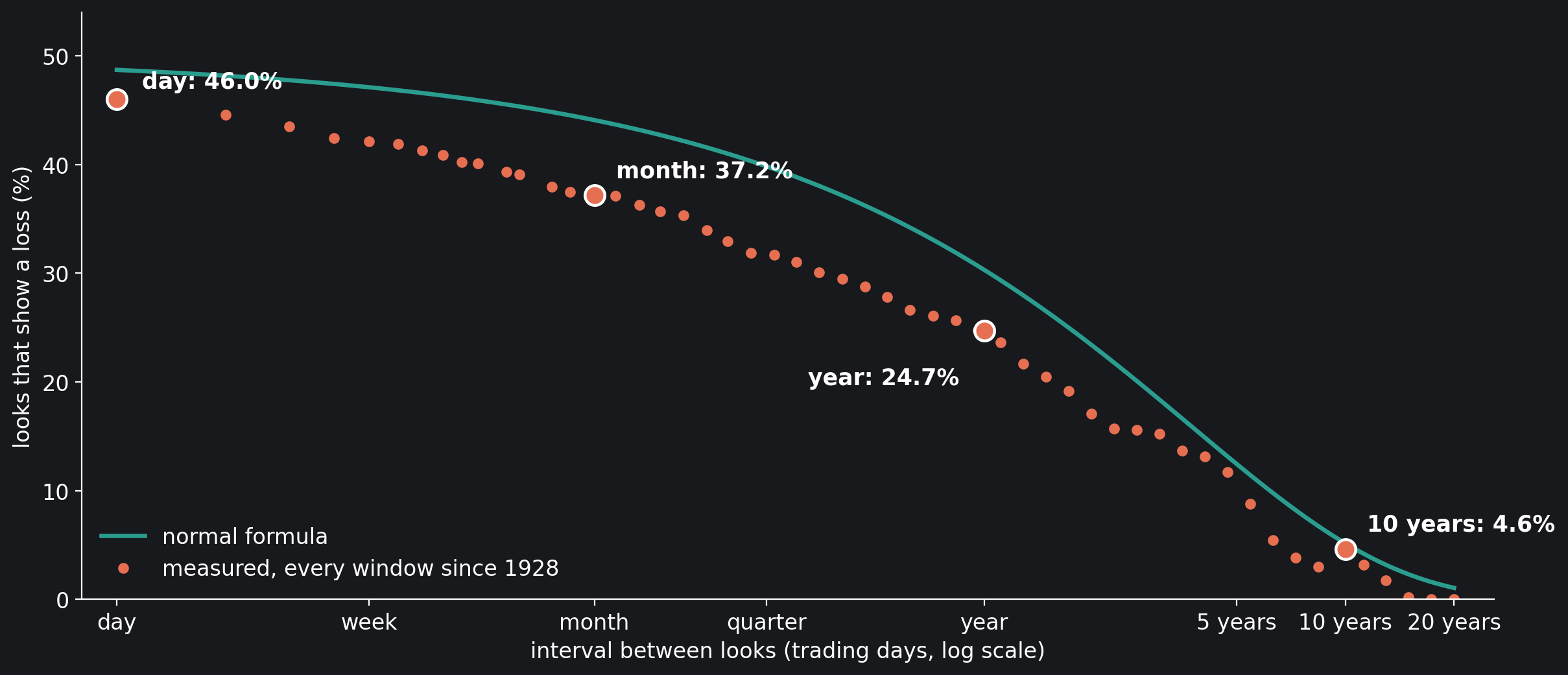
A look every day shows a loss 46.0% of the time, every month 37.2%, every year 24.7% and every ten years 4.6%. No 20-year window since 1928 ended below its start, but the windows overlap: fewer than five separate 20-year spans fit in 98 years, so that 0.0% rests on a handful of independent stretches. The normal formula has the right shape and sits above the measured share at every interval, from 48.7% against 46.0% for a day to 1.1% against none for twenty years. Real daily returns are not normal: their median log return, 0.00063 a day, is above their mean, 0.00039, because a few large falls pull the mean down, so small gains are more common than the formula expects. Figure 1 shows both.
How a Loss Feels
Tversky and Kahneman had 25 graduate students from Berkeley and Stanford choose, gamble after gamble, between a risky prospect and a series of sure amounts, and fitted a value function to each student’s choices. “The median λ was 2.25, indicating pronounced loss aversion.” Score the return $R$ of each look the way such an investor feels it, with a loss weighted $\lambda$ times a gain of the same size,
and average it over every window. A positive average means the looks, taken together, feel like gains; a negative one means the losses outweigh them even though the money grew. Tversky and Kahneman also bent the value function, raising each gain and loss to a power α, whose median “was 0.88 for both gains and losses”; the last column below is that version, as a check.
How a Loss Feels
LAM, ALPHA = 2.25, 0.88

def felt(R, lam=LAM):                  # loss aversion, straight lines
    return np.where(R >= 0, R, lam * R).mean()

def felt_bent(R, lam=LAM, a=ALPHA):    # with the curvature alpha
    return np.where(R >= 0, np.abs(R)**a, -lam * np.abs(R)**a).mean()

print(f"{'look every':<11}{'felt':>9}{'with alpha 0.88':>17}")
for name in ("day", "week", "month", "quarter", "half-year", "year"):
    R = returns_over(LOOKS[name])
    print(f"{name:<11}{felt(R):>+9.4f}{felt_bent(R):>+17.4f}")

# look every      felt  with alpha 0.88
# day          -0.0040          -0.0068
# week         -0.0076          -0.0115
# month        -0.0085          -0.0115
# quarter      +0.0022          +0.0032
# half-year    +0.0242          +0.0296
# year         +0.0783          +0.0889
Looked at every day, every week or every month, stocks feel like a loss: −0.0040, −0.0076, −0.0085. The feeling gets worse from a day to a month before it gets better, because the size of a typical loss grows with the square root of the interval while the drift grows in proportion to it, and at first the square root wins. Looked at every quarter, stocks feel like a small gain, +0.0022; every year, +0.0783. The curvature changes the numbers but not the sign of any of them.
The Break-Even
Somewhere between a month and a quarter the average feeling crosses zero. Since $\max(R,0) = R – \min(R,0)$, the felt value is the plain return plus an extra weight on the losses alone,
so two averages per interval, computed once, give the felt value for any $\lambda$.
The Break-Even
H = np.arange(1, 1261)                 # every interval up to five years
ER = np.array([returns_over(h).mean() for h in H])
EN = np.array([np.minimum(returns_over(h), 0).mean() for h in H])

def measured_break_even(lam):          # the interval after which the
    v = ER + (lam - 1) * EN            # felt value stays above zero
    neg = np.flatnonzero(v < 0)
    if neg.size == 0:
        return 1
    return H[neg[-1]] + 1 if neg[-1] + 1 < H.size else np.nan

bent = np.array([felt_bent(returns_over(h)) for h in H[:252]])
T_meas = measured_break_even(LAM)
print(f"measured break-even, lambda {LAM}: {T_meas} trading days "
      f"({T_meas / 5:.1f} weeks)")
print(f"with alpha {ALPHA}: {np.flatnonzero(bent < 0)[-1] + 2} trading days")

# measured break-even, lambda 2.25: 56 trading days (11.2 weeks)
# with alpha 0.88: 55 trading days
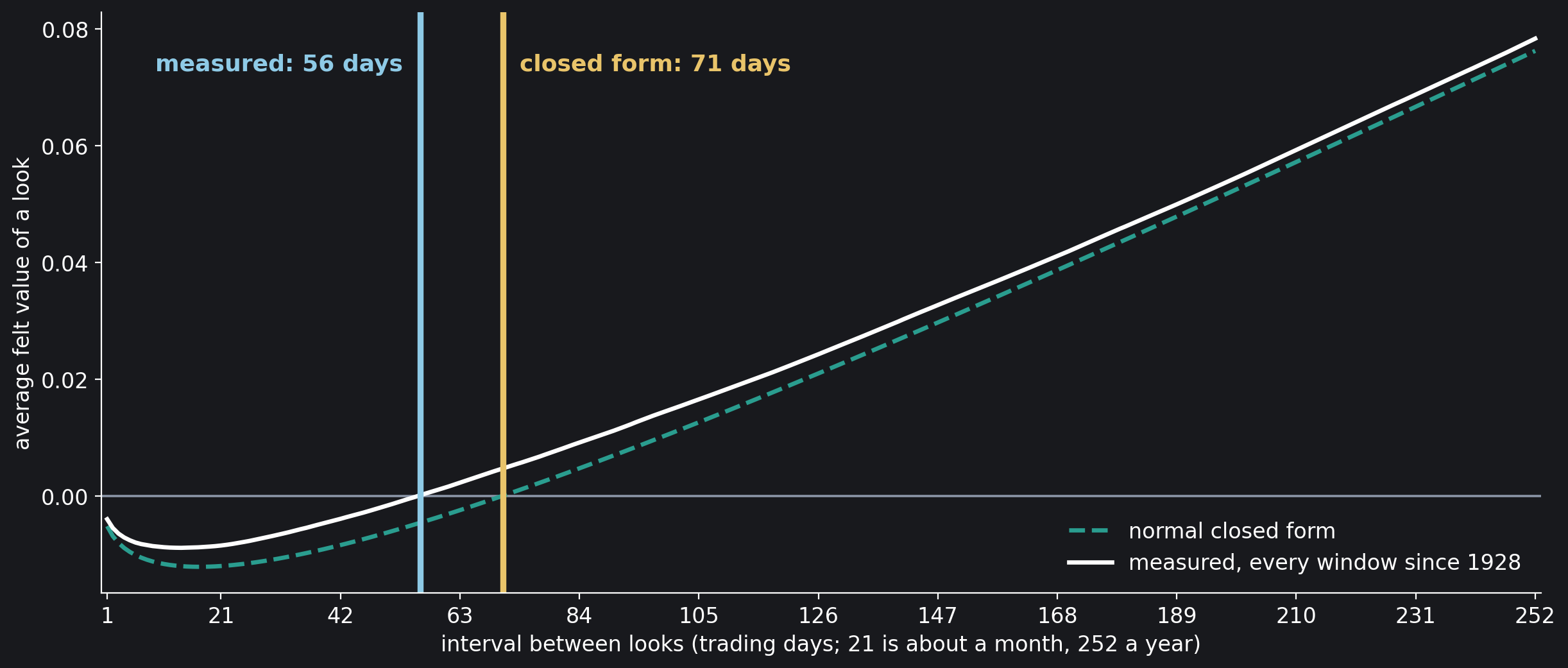
A loss-averse investor with λ = 2.25 feels the S&P 500 as a loss when he looks more often than every 56 trading days, about eleven weeks, and as a gain when he looks less often. The curved value function moves the crossing by one day, to 55.
The Break-Even in Closed Form
Suppose the return over $T$ years is normal with mean $mT$ and spread $\sigma\sqrt{T}$, where $m$ is the mean yearly return, and write $z = mT/(\sigma\sqrt{T})$ for the mean measured in spreads. The normal partial expectation gives the average of the losses alone, and with it the felt value:
with $\varphi$ the normal density. The bracket depends on $z$ and $\lambda$ alone; it is negative at $z = 0$ and rises through zero at a single value $z^*$. With $S = m/\sigma$, the ratio of the market’s mean return to its spread, $z = S\sqrt{T}$, and the felt value crosses zero at
The investor enters only through $z^*$, the market only through $S$.
The Break-Even in Closed Form
from scipy.optimize import brentq

def z_star(lam):                       # the root of the bracket, lam >= 1
    g = lambda z: z + (lam - 1) * (z * norm.cdf(-z) - norm.pdf(z))
    return brentq(g, 0.0, 10.0)

S = m / sigma
zs = z_star(LAM)
T_cf = (zs / S) ** 2
print(f"z* = {zs:.4f}, S = {m:.4f} / {sigma:.4f} = {S:.3f}")
print(f"closed form: {T_cf:.3f} years = {T_cf * DAYS:.0f} trading days")
print(f"measured:    {T_meas / DAYS:.3f} years = {T_meas} trading days")

# z* = 0.3227, S = 0.1155 / 0.1893 = 0.610
# closed form: 0.280 years = 71 trading days
# measured:    0.222 years = 56 trading days
For λ = 2.25, $z^* = 0.3227$. With the market’s $S = 0.610$, the closed form puts the break-even at 0.280 years, 71 trading days; the data put it at 56. The gap is what the normal curve leaves out of the real market, its fat tails and its skew. Figure 2 shows the two curves side by side, and they share their shape: down first, then up through zero.
Your Own λ
Tversky and Kahneman’s 2.25 is a median of 25 students. Put your own value in the first line and run the cell; it gives $z^*$, the closed-form break-even and the measured one, and the same three for five values of λ (any λ of at least 1).
Your Own Lambda
LAMBDA = 2.25          # how much worse a loss feels than an equal gain

zs = z_star(LAMBDA)
print(f"lambda {LAMBDA}: z* = {zs:.4f}, break-even "
      f"{(zs / S) ** 2 * DAYS:.0f} trading days in closed form, "
      f"{measured_break_even(LAMBDA)} measured")
print()
print(f"{'lambda':>7}{'z*':>9}{'closed form':>13}{'measured':>10}")
for lam in (1.5, 2.0, 2.25, 2.5, 3.0):
    z = z_star(lam)
    print(f"{lam:>7.2f}{z:>9.4f}{(z / S) ** 2 * DAYS:>13.0f}"
          f"{measured_break_even(lam):>10}")

# lambda 2.25: z* = 0.3227, break-even 71 trading days in closed form, 56 measured
#
#  lambda       z*  closed form  measured
#    1.50   0.1617           18        13
#    2.00   0.2760           52        40
#    2.25   0.3227           71        56
#    2.50   0.3644           90        74
#    3.00   0.4363          129       115
The more a loss hurts, the longer the gap between looks has to be: 13 trading days for λ = 1.5, 40 for 2, 56 for 2.25, 74 for 2.5 and 115 for 3, measured. The closed form follows the same curve, between 5 and 16 trading days later throughout.
In Real Terms
Benartzi and Thaler gave most weight to nominal returns, because that is how returns are reported. In money of constant value a loss shows more often. Shiller’s consumer price index is monthly, so each month’s inflation is spread evenly over its trading days, and only looks of a month or longer are counted.
In Real Terms
month = df.index.to_period("M")
cpi = df["cpi"].groupby(month).first()
infl = np.log(cpi).diff().fillna(0.0)      # log inflation of each month
per_day = (infl / month.value_counts()).reindex(month).to_numpy()
Lr = np.r_[0.0, np.cumsum(lg - per_day)]   # log wealth after inflation

for name in ("month", "year", "10 years", "20 years"):
    h = LOOKS[name]
    nominal = np.mean(returns_over(h) < 0)
    real = np.mean(Lr[h:] - Lr[:-h] < 0)
    print(f"{name:<9} nominal {nominal:6.1%}   real {real:6.1%}")

# month     nominal  37.2%   real  39.6%
# year      nominal  24.7%   real  29.9%
# 10 years  nominal   4.6%   real  13.6%
# 20 years  nominal   0.0%   real   0.0%
After inflation a monthly look shows a loss 39.6% of the time and a yearly one 29.9%; a look every ten years shows one 13.6% of the time, three times as often as in dollars. No 20-year window lost money after inflation either.
What the Numbers Show
The money and the feeling answer different questions. Over 98 years the market lost on 46% of its days and still turned a dollar into 14,790. A loss-averse investor who looks every day feels that history as a loss; one who looks every quarter feels it as a gain. Between them sits the break-even, 56 trading days in the data and 71 for a normal market with the same mean and spread, and nothing about the market changes there, only the number of looks.
Benartzi and Thaler’s own figure already shows the crossing. In the working-paper version of their Figure 1, built with Tversky and Kahneman’s cumulative prospect theory on monthly CRSP returns from 1926 to 1990, the prospective utility of stocks alone, in nominal terms, is below zero for evaluation periods up to five months and above it from six. What this notebook adds is the measurement day by day over 98 years with dividends, the closed form $T^* = (z^*/S)^2$, which splits the break-even into the investor’s $z^*$ and the market’s $S$, and a cell for your own λ.
Samuelson proved his colleague inconsistent, and under expected utility he was. Benartzi and Thaler read the same answer as a statement about watching: with losses weighted two and a half times, they noted, the colleague “would turn down one bet but accept two or more as long as he didn’t have to watch the bet being played out.” Ninety-eight years of the stock market put a length on the watching: about eleven weeks.
Sources
- P. A. Samuelson, “Risk and Uncertainty: A Fallacy of Large Numbers”, Scientia 98 (1963) 108–113; reprinted in the Casualty Actuarial Society Forum (Spring 1994), from which it is quoted.
- R. Mehra and E. C. Prescott, “The equity premium: A puzzle”, Journal of Monetary Economics 15 (1985) 145–161, doi:10.1016/0304-3932(85)90061-3.
- S. Benartzi and R. H. Thaler, “Myopic Loss Aversion and the Equity Premium Puzzle”, Quarterly Journal of Economics 110 (1995) 73–92, doi:10.2307/2118511. The passage on Samuelson’s colleague and Figure 1 are read in the working paper, NBER Working Paper 4369 (1993), doi:10.3386/w4369.
- A. Tversky and D. Kahneman, “Advances in prospect theory: Cumulative representation of uncertainty”, Journal of Risk and Uncertainty 5 (1992) 297–323, doi:10.1007/BF00122574.
- paveljurke, “S&P 500 (^GSPC) Historical Data”, Kaggle dataset (CC0), daily closes from Yahoo Finance.
- R. J. Shiller, monthly stock market data: S&P Composite price, dividends and the consumer price index, 1871 to the present (ie_data.xls), shillerdata.com.
Every number in this notebook is computed by its own cells from the one data file.
Working on a pricing model or risk system? Let’s talk.