Both Sides of the Policy Get Richer

By Dr. T. Zamrik  ·  October 8, 2026

In a paper he read to the Imperial Academy in St Petersburg, printed in 1738, Daniel Bernoulli asked a question about a merchant he called Caius. Caius, “a Petersburg merchant, has purchased commodities in Amsterdam which he could sell for ten thousand rubles if he had them in Petersburg.” Of every hundred ships that sail from Amsterdam to Petersburg at that time of year, five are usually lost, and nobody will insure the cargo for less than 800 rubles, “an amount which he considers outrageously high.” Should he insure?

By expected value, the merchant should never pay that price: the fair premium, the expected loss, is 500 rubles, so the policy costs him 300 rubles a voyage on average, and whatever he loses the insurer gains. Bernoulli’s answer was different. A merchant worth less than 5,043 rubles should buy the policy, and an insurer worth more than 14,243 should sell it, so both sign, and both are right.

This notebook computes Bernoulli’s two numbers, shows why expected value calls insurance a zero-sum transfer and why growth over time does not, simulates 10,000 shipowners over 500 voyages, and maps who gains at every fortune and price.

Bernoulli’s Merchant

Bernoulli valued a fortune by its logarithm: a gain is worth less the more one already has. The merchant, worth $W$ besides the cargo, insures if his certain fortune with the policy is worth more than his gamble without it, and an insurer worth $Y$ sells if the policy raises the value of his own fortune:

with the cargo $G = 10{,}000$ rubles, the chance of loss $p = 5\%$ and the premium $F = 800$ rubles. Each inequality turns into an equality at one fortune, and a root-finder finds it.

import numpy as np
from scipy.optimize import brentq

G, p, F = 10_000, 0.05, 800          # cargo, chance of loss, premium (rubles)

def merchant_gain(W, F=F):           # log value insured minus uninsured
    return np.log(W + G - F) - ((1 - p) * np.log(W + G) + p * np.log(W))

def insurer_gain(Y, F=F):            # log value of selling minus not selling
    return (1 - p) * np.log(Y + F) + p * np.log(Y + F - G) - np.log(Y)

W_star = brentq(merchant_gain, 1, 1e6)
Y_star = brentq(insurer_gain, G - F + 1e-6, 1e8)
print(f"fair premium p*G: {p * G:,.0f} rubles")
for prem in (800, 600):
    w = brentq(merchant_gain, 1, 1e6, args=(prem,))
    y = brentq(insurer_gain, G - prem + 1e-6, 1e8, args=(prem,))
    print(f"premium {prem}: merchant insures below {w:,.0f}, "
          f"insurer sells above {y:,.0f}")

# fair premium p*G: 500 rubles
# premium 800: merchant insures below 5,042, insurer sells above 14,242
# premium 600: merchant insures below 20,478, insurer sells above 29,878

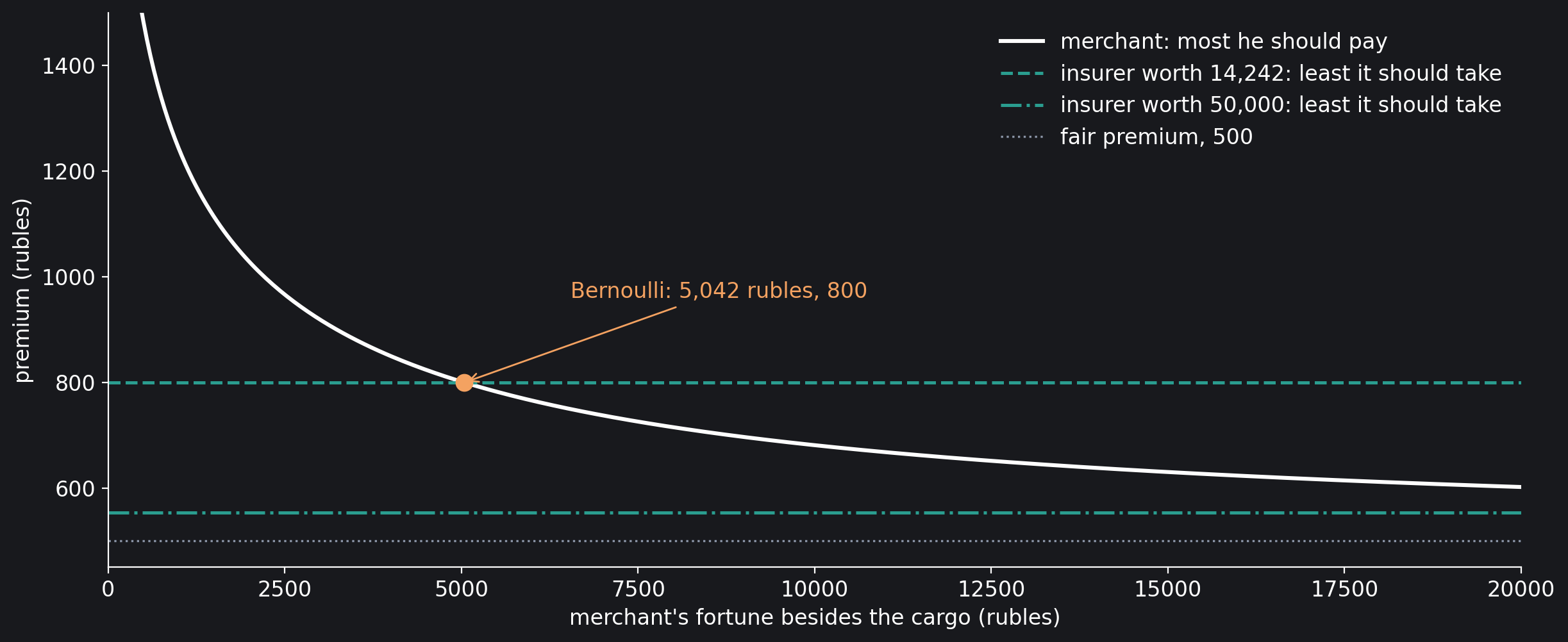
Bernoulli’s numbers come back to the ruble: 5,042 and 14,242, which he rounded up to 5,043 and 14,243, and at a premium of 600 rubles, 20,478 and 29,878, as he wrote. A poor merchant and a rich insurer both gain from a policy priced 60% above its expected cost.

One Contract, Two Answers

In expectation the contract is zero-sum. The insurer expects to collect $F – pG$, 300 rubles, and the merchant expects to pay exactly that, so if expected value were the measure, one side would be making a mistake. Bernoulli’s logarithm looks like a matter of taste, a utility function that happens to make both sides happy.

In 2015 Ole Peters and Alexander Adamou of the London Mathematical Laboratory read it differently. Their paper, revised in 2017 as “Insurance makes wealth grow faster”, argues that “the puzzle goes away if contracts are evaluated by their effect on the time-average growth rate of wealth”: the logarithm is not a taste but the rate at which one merchant’s wealth actually grows if he does this again and again. John Kelly had said the same of a gambler in 1956: the logarithm matters because it “is additive in repeated bets and to which the law of large numbers applies.” The example below is theirs.

The Same Voyage, Repeated

Make the voyage repeat. In Peters and Adamou’s example a shipowner worth 100,000 dollars makes 4,000 on each voyage, 4% of his wealth, on every voyage that arrives and loses a ship worth 30,000, 30% of it, on one voyage in twenty. He can insure with a company ten times richer, which pays him the lost gain and the ship, 34% of his wealth, when the ship sinks, for a fee $f$ of his wealth every voyage; theirs is 1,800, or 1.8%. Per voyage, the two ways of scoring the uninsured owner are

with $g = 4\%$, $c = 30\%$ and $p = 5\%$. Insured, he multiplies his wealth by $\textstyle 1 + g – f$ every voyage, whatever the sea does.

g, c, p = 0.04, 0.30, 0.05     # gain, ship, chance of loss (shares of wealth)
L, ratio = g + c, 0.10         # insurer pays L; owner is 1/10 of insurer
f = 0.018                      # the fee: 1,800 on a wealth of 100,000

def owner_growth(f=None):
    if f is None:              # uninsured
        return (1 - p) * np.log1p(g) + p * np.log1p(-c)
    return np.log1p(g - f)

def insurer_growth(f, ratio=ratio):
    return (1 - p) * np.log1p(ratio * f) + p * np.log1p(ratio * (f - L))

print(f"owner, expected multiplier:  uninsured {(1-p)*(1+g)+p*(1-c):.4f}"
      f"  insured {1 + g - f:.4f}")
print(f"owner, growth per voyage:    uninsured {owner_growth():.5f}"
      f"  insured {owner_growth(f):.5f}")
print(f"insurer, growth per voyage:  {insurer_growth(f):.6f}")

# owner, expected multiplier:  uninsured 1.0230  insured 1.0220
# owner, growth per voyage:    uninsured 0.01943  insured 0.02176
# insurer, growth per voyage:  0.000072

By expected value the owner should not insure: uninsured, his wealth is multiplied by 1.0230 on average, insured by 1.0220. By growth he should: uninsured his wealth grows 0.01943 a voyage on the logarithmic scale, insured 0.02176, 12% faster. And the insurer’s own growth, 0.000072 a voyage, is positive too.

The two growth rates set a window of fees. The owner gains from any fee below the one at which insured and uninsured growth are equal, and the insurer from any fee above the one at which its growth is zero:

f_max = brentq(lambda f: owner_growth(f) - owner_growth(), 0, g)
f_min = brentq(insurer_growth, 0, L)
print(f"fair fee, p*(g+c):       {p * L:.3%} of the owner's wealth")
print(f"insurer gains above:     {f_min:.3%}")
print(f"owner gains below:       {f_max:.3%}")

# fair fee, p*(g+c):       1.700% of the owner's wealth
# insurer gains above:     1.728%
# owner gains below:       2.038%

Any fee from 1.728% to 2.038% of the owner’s wealth makes both grow faster. The fair fee, 1.700%, is below the window: an insurer charging the fair price would shrink, because its losses come in lumps and the logarithm punishes lumps. At the window’s top the owner pays 20% over the fair fee and still grows faster than without the policy.

10,000 Owners, 500 Voyages

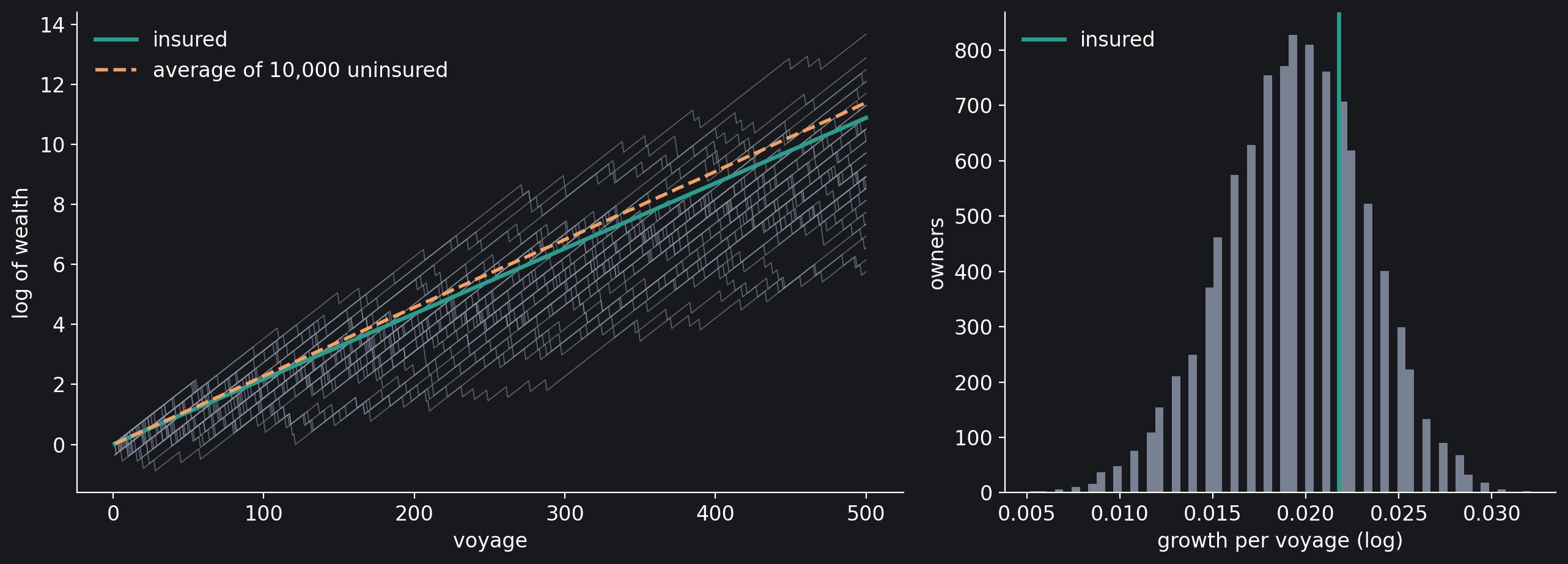
The growth rate is what one owner experiences over many voyages; the expected multiplier is what the average of many owners does. Simulate 10,000 uninsured owners for 500 voyages each and set them against one insured owner, whose path is certain.

rng = np.random.default_rng(20261008)
N, T = 10_000, 500
sunk = rng.random((N, T)) < p                  # True where a ship was lost
steps = np.where(sunk, np.log1p(-c), np.log1p(g))
logW = steps.cumsum(axis=1)                    # log wealth, starting at 0
rate = logW[:, -1] / T                         # each owner's growth rate
ins = owner_growth(f)

lo, hi = np.quantile(rate, [0.05, 0.95])
print(f"uninsured growth per voyage: median {np.median(rate):.5f}, "
      f"middle 90% {lo:.5f} to {hi:.5f}")
print(f"insured growth per voyage:   {ins:.5f}")
print(f"uninsured owners who grew slower than the insured one: "
      f"{np.mean(rate < ins):.1%}")
print(f"wealth after 500 voyages, average of the 10,000: "
      f"{np.exp(logW[:, -1]).mean():,.0f} times")
print(f"wealth after 500 voyages, the median owner:      "
      f"{np.exp(np.median(logW[:, -1])):,.0f} times")
print(f"wealth after 500 voyages, insured:               "
      f"{np.exp(ins * T):,.0f} times")

# uninsured growth per voyage: median 0.01943, middle 90% 0.01309 to 0.02576
# insured growth per voyage:   0.02176
# uninsured owners who grew slower than the insured one: 68.8%
# wealth after 500 voyages, average of the 10,000: 88,607 times
# wealth after 500 voyages, the median owner:      16,531 times
# wealth after 500 voyages, insured:               53,143 times

The typical uninsured owner grows at 0.01943 a voyage and the insured one at 0.02176, and 68.8% of the 10,000 uninsured owners grew slower than the insured one. Yet the average wealth of the 10,000 after 500 voyages, 88,607 times what they started with, is well above the insured owner’s 53,143: a few owners who rarely lost a ship pull the average up, while the median uninsured owner ends with 16,531 times. The expected value describes that average, and no single owner lives it.

The Insurer Needs Many Policies

The insurer’s growth is positive but small, and a single policy is a lump. An insurer that writes one policy a voyage, each a tenth of its size, can still shrink over 500 voyages; one a thousand times richer than each owner that writes a hundred independent policies a voyage carries the same total size, ten owners’ worth, in many small pieces.

def insurer_paths(k, ratio_each, n=4_000, T=500, seed=1):
    r = np.random.default_rng(seed)
    claims = r.binomial(k, p, size=(n, T))    # ships lost in a voyage
    mult = 1 + ratio_each * (k * f - claims * L)
    return np.log(mult).sum(axis=1) / T       # growth per voyage

for k, ratio_each in ((1, 0.10), (100, 0.001)):
    r = insurer_paths(k, ratio_each)
    print(f"{k:3d} policies a voyage: median growth {np.median(r):.6f}, "
          f"insurers that shrank {np.mean(r < 0):.1%}")

#   1 policies a voyage: median growth 0.000072, insurers that shrank 36.1%
# 100 policies a voyage: median growth 0.000100, insurers that shrank 0.1%

Writing one policy a voyage, 36.1% of insurers still shrank over 500 voyages, though the median grew. Writing a hundred small independent policies, the same insurer’s growth rose to 0.000100 a voyage, the whole expected margin of 0.1% of the owner’s wealth on a tenth-sized book, and only 0.1% of 4,000 insurers shrank. Pooling turns the insurer’s expected value into its actual growth. It is the business that began in the coffee house of Edward Lloyd in London, first recorded in 1688 and “popular with ship owners and captains.” Bernoulli saw the limit too: “no one, however rich, would be managing his affairs properly if he individually undertook the insurance for less than five hundred rubles”, the fair premium.

Who Should Insure

Back to Bernoulli’s merchant. For each fortune the merchant’s highest acceptable premium solves his equation, and for each fortune of the insurer the lowest acceptable premium solves the insurer’s. The poorer the merchant, the more he should be willing to pay; the richer the insurer, the closer to the fair 500 rubles it can go.

What It Means

Expected value answers a question about a crowd: the average of many merchants, each shipping once. A merchant ships again and again, and what he lives through is the growth along his own path, which is what Bernoulli’s logarithm measures. The two differ because a loss takes a share of whatever wealth is left, so along one path gains and losses do not average out the way they do across a crowd. On that measure an insurance contract is not a transfer from one side to the other. The buyer pays for a smoother path and grows faster; the seller, richer and pooling many policies, turns the premium into growth with almost no risk. Bernoulli reached the conclusion in 1738: insurance “offers advantages to all persons concerned.”

Peters has since argued, in Nature Physics in 2019, that economics often uses expected values where time averages belong; in the same journal in 2020, Doctor, Wakker and Wang replied that expected-utility theory already allows for it. The arithmetic here does not depend on who is right: with Bernoulli’s numbers or with Peters and Adamou’s, a policy priced above its expected cost makes both sides grow faster.

Sources

1. D. Bernoulli, “Specimen theoriae novae de mensura sortis”, Commentarii Academiae Scientiarum Imperialis Petropolitanae 5 (1738) 175–192; translated by L. Sommer as “Exposition of a new theory on the measurement of risk”, Econometrica 22 (1954) 23–36, §15.
2. O. Peters and A. Adamou, “Insurance makes wealth grow faster”, arXiv:1507.04655 (2017; first version 2015).
3. J. L. Kelly Jr., “A new interpretation of information rate”, Bell System Technical Journal 35 (1956) 917–926.
4. Lloyd’s, “Coffee and commerce”, lloyds.com: Edward Lloyd’s coffee house, first recorded in 1688.
5. O. Peters, “The ergodicity problem in economics”, Nature Physics 15 (2019) 1216–1221.
6. J. N. Doctor, P. P. Wakker and T. V. Wang, “Economists’ views on the ergodicity problem”, Nature Physics 16 (2020) 1168.

Every number in this notebook is computed by its own cells; nothing is loaded from outside.

Working on a pricing model or risk system? Let’s talk.