
The Babylonian Talmud has a rule for money, in tractate Bava Metzia, folio 42a. Rabbi Yitzḥak says: “A person should always divide his money into three; [he should bury] one-third in the ground, and [invest] one-third in business, and [keep] one-third in his possession.” Land, trade and cash at hand, in equal shares, whatever each of them promised. In the language of this notebook it is the 1/N rule, with N = 3.
In 1952 Harry Markowitz replaced the rule with a calculation. His paper “Portfolio Selection”, in the Journal of Finance, judged a portfolio by two numbers, its expected return and its variance, and the variance of a portfolio depends on how every pair of its holdings moves together. The rule that grew out of it says how much to hold of each asset: in proportion to $\Sigma^{-1}\mu$, the inverse of the covariance matrix of the returns times the vector of their expected values. It became modern portfolio theory, and in 1990 Markowitz shared the Nobel prize in economics with Merton Miller and William Sharpe “for their pioneering work in the theory of financial economics.”
His own pension went another way. Soon after the paper he had to decide how to split his contributions between a bond fund and a stock fund, and he described the decision to the journalist Jason Zweig in 1997: “I should have computed the historical co-variances of the asset classes and drawn an efficient frontier. Instead, I visualized my grief if the stock market went way up and I wasn’t in it–or if it went way down and I was completely in it. My intention was to minimize my future regret. So I split my contributions 50/50 between bonds and equities.” That was 1952, he made clear in 2009, and it did not last: “Now I don’t do that.”
In 2009 Victor DeMiguel, Lorenzo Garlappi and Raman Uppal put the two rules side by side. Their paper opens with the Talmud’s sentence. It then sets the sample-based Markowitz rule and its “extensions designed to reduce estimation error” against 1/N: “Of the 14 models we evaluate across seven empirical datasets, none is consistently better than the 1/N rule in terms of Sharpe ratio, certainty-equivalent return, or turnover.” They also worked out how much history the Markowitz rule would need before it won: “around 3000 months for a portfolio with 25 assets and about 6000 months for a portfolio with 50 assets”, which is 250 and 500 years. Two years later Jun Tu and Guofu Zhou titled their follow-up “Markowitz meets Talmud”.
This notebook runs the contest again, three ways: on 1,000 random portfolios of 25 stocks from the S&P 500, 2013 to 2018; on 57 years of 48 industry portfolios with dividends, which include the seventeen years since the paper was printed, a test of the paper on data it never saw; and in closed form, to see why the answer comes out as it does.
Two Data Files
The first file holds the daily returns of 459 members of the S&P 500 with a price on every trading day from 8 February 2013 to 7 February 2018, cut from a public-domain Kaggle dataset; they are price returns, without dividends. The second holds the monthly returns of Kenneth French’s 48 industry portfolios of US stocks, value-weighted and with dividends, from July 1969 to August 2026, and the one-month Treasury bill rate from his factor file. Every strategy is judged on excess returns, its return minus the T-bill’s; for the stocks, each day gets a 21st of its month’s T-bill return, a month having about 21 trading days.
Two Data Files
import numpy as np
import pandas as pd

rets = pd.read_csv("data/sp500_returns.csv", index_col="date",
                   parse_dates=True)
ind = pd.read_csv("data/french_48_industries.csv", index_col="month")
R = np.expm1(rets.to_numpy())          # simple daily returns, 459 stocks
rf_m = ind["RF"]                       # the one-month T-bill, by month
rf_d = rf_m[rets.index.strftime("%Y-%m")].to_numpy() / 21   # per day
X = ind.drop(columns="RF").to_numpy()  # 48 industries, monthly
rf_i = rf_m.to_numpy()
print(f"stocks: {R.shape[1]}, {len(R):,} trading days, "
      f"{rets.index[0]:%d %b %Y} to {rets.index[-1]:%d %b %Y}")
print(f"industries: {X.shape[1]}, {len(X)} months, "
      f"{ind.index[0]} to {ind.index[-1]}")
print(f"T-bill: {rf_m['2014-02':'2018-01'].mean() * 12:.2%} a year in "
      f"2014-18, {rf_i.mean() * 12:.2%} over 1969-2026")

# stocks: 459, 1,258 trading days, 11 Feb 2013 to 07 Feb 2018
# industries: 48, 686 months, 1969-07 to 2026-08
# T-bill: 0.28% a year in 2014-18, 4.36% over 1969-2026
Six Ways to Split the Money
At every rebalance each strategy is rebuilt from a window of the last $M$ observations of excess returns, with $\hat\mu$ their average and $\hat\Sigma$ their sample covariance matrix. Five of the six can be followed in real time; the sixth cheats.
- 1/N: $1/N$ in each asset.
- Markowitz, textbook: $x = \hat\Sigma^{-1}\hat\mu$, scaled to $w = x / \lvert\mathbf{1}^\top x\rvert$.
- Markowitz, long-only: the mix with the highest Sharpe ratio among $w \ge 0$, $\mathbf{1}^\top w = 1$.
- Minimum variance, shrinkage: $w \propto \hat\Sigma_{LW}^{-1}\mathbf{1}$, with Ledoit and Wolf’s shrunk covariance matrix.
- Minimum variance, long-only: the mix with the lowest variance among $w \ge 0$, $\mathbf{1}^\top w = 1$.
- Markowitz, hindsight: the textbook rule, computed once from the whole sample. Not investable.
The scaling of the textbook rule is DeMiguel, Garlappi and Uppal’s: dividing by the absolute value of the sum keeps the direction of the position when the weights add up to a negative number, and whatever $w$ leaves over sits in T-bills. The minimum-variance rules never look at $\hat\mu$. Ledoit and Wolf’s estimator pulls the sample covariance matrix part of the way towards a multiple of the identity, by an amount estimated from the data.
The two long-only rules are small quadratic programmes, and both are solved here as one non-negative least-squares problem:
with $a = \mathbf{1}$ for the lowest variance and $a = \hat\mu$ for the highest Sharpe ratio, which is the smallest $y^\top\hat\Sigma y$ with $\hat\mu^\top y = 1$. Because $y \ge 0$ is a cone and $y^\top\hat\Sigma y$ grows with the square of $y$, the penalised minimiser is a multiple of the constrained one, so the rescaled weights are exact for any $\lambda > 0$.
The Long-Only Solver
from scipy.optimize import nnls

def long_only(S, a):     # min y'Sy, a'y = 1, y >= 0; w = y / sum(y)
    n = len(a)
    L = np.linalg.cholesky(S / np.diag(S).mean() + 1e-12 * np.eye(n))
    A = np.vstack([L.T, 100 * a / np.abs(a).max()])   # lambda = 100**2
    b = np.r_[np.zeros(n), 100.0]
    y = nnls(A, b, maxiter=50 * n)[0]
    return y / y.sum()

E0 = (X - rf_i[:, None])[:60]          # 48 industries, Jul 1969 - Jun 1974
w = long_only(np.cov(E0.T), np.ones(48))
print(f"lowest-variance long-only mix, 1969-74: {np.sum(w > 1e-6)} of 48 "
      f"industries held, the largest {ind.columns[w.argmax()]} {w.max():.0%}")

# lowest-variance long-only mix, 1969-74: 7 of 48 industries held, the largest Telcm 31%
Six Ways to Split the Money
from sklearn.covariance import ledoit_wolf

def weights(E):                        # E: a window of excess returns
    n = E.shape[1]
    mu, S, one = E.mean(0), np.cov(E.T), np.ones(n)
    x = np.linalg.solve(S, mu)
    z = np.linalg.solve(ledoit_wolf(E)[0], one)
    return {"ew": one / n, "mv": x / abs(x.sum()),
            "mv_long": long_only(S, mu if (mu > 0).any() else one),
            "min_lw": z / z.sum(), "min_long": long_only(S, one)}

def hindsight(E):                      # the textbook rule, whole sample
    x = np.linalg.solve(np.cov(E.T), E.mean(0))
    return x / abs(x.sum())

KEYS = ["ew", "mv", "mv_long", "min_lw", "min_long", "mv_hind"]
NAMES = dict(zip(KEYS, ["1/N", "Markowitz, textbook", "Markowitz, long-only",
                        "Min variance, shrinkage", "Min variance, long-only",
                        "Markowitz, hindsight"]))
W0 = dict(weights(E0), mv_hind=hindsight(X - rf_i[:, None]))
print(f"{'1969-74 window':25}{'lowest':>8}{'highest':>9}{'longs + shorts':>16}")
for k, w in W0.items():
    print(f"{NAMES[k]:25}{w.min():8.0%}{w.max():9.0%}{np.abs(w).sum():16,.0%}")

# 1969-74 window             lowest  highest  longs + shorts
# 1/N                            2%       2%            100%
# Markowitz, textbook          -82%      99%          1,418%
# Markowitz, long-only           0%      60%            100%
# Min variance, shrinkage      -24%      26%            417%
# Min variance, long-only        0%      31%            100%
# Markowitz, hindsight         -66%      54%          1,035%
Over the industries’ first five years the textbook rule’s long and short positions add up to 14 times the capital; shrinkage cuts that to 4 times, and the long-only lowest-variance mix holds just 7 of the 48 industries. (The hindsight row uses all 57 years.)
Before trusting the solver, a check against a general one: the same two problems, as stated (the lowest variance, and the highest Sharpe ratio, each over $w \ge 0$ with $\mathbf{1}^\top w = 1$), handed to SciPy’s SLSQP on ten random 250-day windows of 25 stocks and ten random 60-month windows of the 48 industries.
A Check on the Solver
from scipy.optimize import minimize

def slsqp(S, a, sharpe):               # the same problems, solved directly
    n, S, a = len(a), S / np.diag(S).mean(), a / np.abs(a).max()
    f = ((lambda w: -(a @ w) / np.sqrt(w @ S @ w)) if sharpe
         else (lambda w: w @ S @ w))
    w = minimize(f, np.full(n, 1 / n), method="SLSQP",
                 bounds=[(0, None)] * n, options={"ftol": 1e-15,
                 "maxiter": 2000}, constraints={"type": "eq",
                 "fun": lambda w: w.sum() - 1}).x
    return w / w.sum()

rng = np.random.default_rng(7)
gap = []
for E, M, n in [(R - rf_d[:, None], 250, 25)] * 10 + [(X, 60, 48)] * 10:
    t = rng.integers(M, len(E))
    W = E[t - M:t, rng.choice(E.shape[1], n, replace=False)]
    mu, S = W.mean(0), np.cov(W.T)
    for a, sharpe in ((mu, True), (np.ones(n), False)):
        if mu.max() > 0 or not sharpe:
            gap.append(np.abs(long_only(S, a) - slsqp(S, a, sharpe)).max())
print(f"{len(gap)} problems; largest weight difference {max(gap):.0e}")

# 40 problems; largest weight difference 8e-08
The two solvers agree to better than one part in a million in every weight.
A Thousand Portfolios of 25 Stocks
Each random portfolio draws 25 of the 459 stocks. The first 250 trading days, about a year, are the first estimation window; from then on, every 21 trading days each strategy is re-estimated from the last 250 days and rebalanced, from February 2014 to February 2018. Between rebalances the holdings drift with their prices, and whatever the weights leave over earns the T-bill rate. A strategy whose capital touches zero is wiped out: it stays at zero, it gets no Sharpe ratio, and it counts as a loss to 1/N. The Sharpe ratio is the mean daily excess return over its standard deviation, times $\sqrt{252}$.
One Portfolio, Six Ways
def backtest(r, rf, M, H=21):          # r: simple returns, rf: T-bill's
    E = r - rf[:, None]                # excess returns
    W_h = hindsight(E)
    ex, turn = {k: [] for k in KEYS}, {k: [] for k in KEYS}
    cap, held = dict.fromkeys(KEYS, 1.0), dict.fromkeys(KEYS)
    for s in range(M, len(r), H):      # rebalance every H days
        W = dict(weights(E[s - M:s]), mv_hind=W_h)
        g = np.cumprod(1 + r[s:s + H], 0)      # each asset's growth
        gc = np.cumprod(1 + rf[s:s + H])       # the cash's growth
        for k in KEYS:
            v = (1 - W[k].sum()) * gc + g @ W[k]   # 1 put in at day s
            if cap[k] == 0 or (v <= 0).any():
                cap[k] = 0.0           # wiped out, and it stays out
                continue
            if held[k] is not None:    # trading = new weights - drifted
                turn[k].append(np.abs(W[k] - held[k]).sum())
            ex[k].append(v / np.r_[1, v[:-1]] - 1 - rf[s:s + H])
            held[k], cap[k] = W[k] * g[-1] / v[-1], cap[k] * v[-1]
    return ex, cap, turn

ex, cap, turn = backtest(R[:, :25], rf_d, 250)   # the first 25 tickers
print("the first 25 tickers, what a dollar became:")
print(", ".join(f"{k} {cap[k]:.2f}" for k in KEYS))

# the first 25 tickers, what a dollar became:
# ew 1.58, mv 0.00, mv_long 1.14, min_lw 1.43, min_long 1.41, mv_hind 4.08
A Thousand Portfolios
def stocks_study(n_stocks=25, window=250, draws=1000, seed=20261011):
    rng = np.random.default_rng(seed)
    rows = {k: [] for k in KEYS}
    for _ in range(draws):
        pick = rng.choice(R.shape[1], n_stocks, replace=False)
        ex, cap, turn = backtest(R[:, pick], rf_d, window)
        for k in KEYS:
            e = np.concatenate(ex[k] or [np.zeros(2)])
            sharpe = e.mean() / e.std() * np.sqrt(252) if cap[k] else np.nan
            rows[k].append([sharpe, cap[k], e.std() * np.sqrt(252),
                            np.mean(turn[k]) if turn[k] else np.nan])
    cols = ["sharpe", "wealth", "vol", "turnover"]
    return {k: pd.DataFrame(v, columns=cols) for k, v in rows.items()}

stocks = stocks_study()
print(f"{len(stocks['ew']):,} portfolios of 25 stocks, tested from "
      f"{rets.index[250]:%d %b %Y} to {rets.index[-1]:%d %b %Y}")

# 1,000 portfolios of 25 stocks, tested from 07 Feb 2014 to 07 Feb 2018
The Scoreboard
def scoreboard(res):
    ew = res["ew"]["sharpe"]
    print(f"{'':25}{'median':>8}{'1 became':>10}{'wiped':>8}{'beats':>8}"
          f"{'traded':>9}\n{'':25}{'Sharpe':>8}{'(median)':>10}{'out':>8}"
          f"{'1/N':>8}{'a month':>9}")
    for k, d in res.items():
        wiped = d["sharpe"].isna()
        med = d["sharpe"].fillna(-np.inf).median()
        sh = f"{med:8.2f}" if np.isfinite(med) else f"{'wiped':>8}"
        beat = np.mean(~wiped & (d["sharpe"] > ew))
        print(f"{NAMES[k]:25}{sh}{d['wealth'].median():10.2f}"
              f"{wiped.mean():8.1%}{'' if k == 'ew' else f'{beat:.1%}':>8}"
              f"{d['turnover'].median():9,.0%}")

scoreboard(stocks)

#                            median  1 became   wiped   beats   traded
#                            Sharpe  (median)     out     1/N  a month
# 1/N                          0.89      1.56    0.0%               4%
# Markowitz, textbook         wiped      0.00   86.2%    1.7%   1,098%
# Markowitz, long-only         0.59      1.40    0.0%   14.9%      58%
# Min variance, shrinkage      0.85      1.45    0.0%   44.5%      32%
# Min variance, long-only      0.82      1.42    0.0%   39.2%      22%
# Markowitz, hindsight         2.28      8.90    0.0%  100.0%      34%
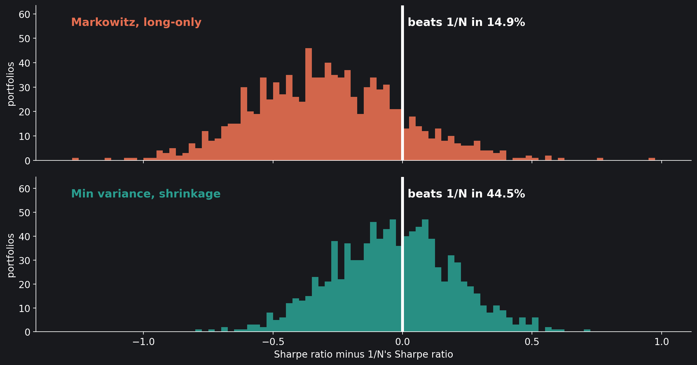
The textbook rule wiped out 862 of the 1,000 portfolios and beat 1/N in 17. Its long-only version survived everywhere but beat 1/N in only 149, with a median Sharpe ratio of 0.59 against 1/N’s 0.89. The two minimum-variance rules, which ignore the means, came close: shrinkage beat 1/N in 445 portfolios and long-only in 392, with median Sharpe ratios of 0.85 and 0.82. And the textbook rule computed with hindsight, from the whole five years’ means and covariances, beat 1/N in all 1,000 with a median Sharpe ratio of 2.28, two and a half times 1/N’s, turning a dollar into 8.90 where 1/N made 1.56.
Trading costs are left out, and they would only widen the gaps: 1/N trades 4% of its capital a month to get back to equal weights, the other investable rules between 22% and 58%, the textbook rule 1,098% until its capital runs out. These stocks are also 459 survivors of five years, 2013 to 2018, a single bull-market sample. Figure 1 shows the whole spread for long-only Markowitz and shrinkage minimum variance.
Why the Means Poison It
A window of 250 days is one year of data. Slice the year into as many days as you like: the standard error of an estimated average annual return after $Y$ years is $\sigma/\sqrt{Y}$, with $\sigma$ the annual volatility, because only the start and end of the period carry information about the drift. A volatility is different: it is estimated from the number of observations, to about $\sigma/\sqrt{2n}$ from $n$ daily returns.
Why the Means Poison It
vol = R.std(0) * np.sqrt(252)          # each stock's annual volatility
s = np.median(vol)
print(f"the median stock's volatility: {s:.1%} a year")
print(f"{'years of data':>13}{'its mean, to within':>22}"
      f"{'its volatility, to within':>28}")
for years in (1, 5, 100):
    print(f"{years:>13}{'±':>14}{s / np.sqrt(years):.1%} a year"
          f"{'±':>14}{s / np.sqrt(2 * 252 * years):.1%} a year")

# the median stock's volatility: 22.6% a year
# years of data   its mean, to within   its volatility, to within
#             1             ±22.6% a year             ±1.0% a year
#             5             ±10.1% a year             ±0.5% a year
#           100             ±2.3% a year             ±0.1% a year
One year of the median stock, whose volatility is 22.6% a year, pins its expected return to within ±22.6 points, one standard error: an estimate of 10% a year is as consistent with −13% as with 33%. The whole five years of the file narrow it to ±10.1 points; a century of data would narrow it to ±2.3. The same single year of daily data pins the volatility to within ±1.0 point. The textbook rule multiplies the well-measured covariances’ inverse into the badly measured means and bets hard on whatever the noise says; the minimum-variance rules use only the part that is measured well.
The stocks are price returns, without dividends. Could dividends rescue long-only Markowitz? The extra return a year it would need to match 1/N’s Sharpe ratio is the Sharpe gap times its own volatility:
What Dividends Would Have to Do
ew = stocks["ew"]
print(f"{'':25}{'median volatility':>18}{'extra return needed':>21}")
for k in ("mv_long", "min_lw", "min_long"):
    d = stocks[k]
    need = (ew["sharpe"] - d["sharpe"]) * d["vol"]   # a year
    print(f"{NAMES[k]:25}{d['vol'].median():18.1%}{need.median():21.1%}")

#                           median volatility  extra return needed
# Markowitz, long-only                  16.0%                 4.9%
# Min variance, shrinkage               11.1%                 0.4%
# Min variance, long-only               11.1%                 0.7%
Long-only Markowitz would need 4.9 points a year more than it earned, the median over the 1,000 portfolios. For dividends to supply that, the stocks it favours would have to out-yield 1/N’s, drawn from the same 25 names, by 4.9 points a year: more than twice the dividend yield of the whole S&P 500 in those years, about 2%. The minimum-variance rules need 0.4 and 0.7 points a year, and a gap of that size dividends could close or widen. Those close calls are for the second data set, which carries its dividends.
Fifty-Seven Years of Industries
DeMiguel, Garlappi and Uppal’s industry data were French’s 10 industries, to November 2004. Here are his 48, every one with a return in every month from July 1969 to August 2026. Each month the strategies are re-estimated from the last 60 months, five years, the length the paper calls typical, so the first portfolio is held in July 1974. The second column starts again from a dollar in January 2009, the year the paper was printed, and runs on data the paper never saw. A Sharpe ratio here is computed from the series of monthly excess returns, as the paper computes it, and annualised by $\sqrt{12}$; for the textbook rule that is the only way to get one, because its capital does not survive.
Month by Month
def industries(M):                     # the six, rebalanced every month
    E = X - rf_i[:, None]
    W_h = hindsight(E)
    rows = [{k: w @ E[t] for k, w in
             dict(weights(E[t - M:t]), mv_hind=W_h).items()}
            for t in range(M, len(E))]
    return pd.DataFrame(rows, index=ind.index[M:])[KEYS]

def summary(ex):                       # Sharpe, growth of 1, month of ruin
    g = 1 + ex.add(rf_m[ex.index], axis=0)
    dead = g.le(0).cummax()
    wealth = g.cumprod().mask(dead, 0.0)
    ruin = dead.idxmax().where(dead.any(), "")
    return ex.mean() / ex.std(ddof=0) * np.sqrt(12), wealth, ruin

ind60 = industries(60)
print(f"{len(ind60)} months of returns for each strategy, "
      f"{ind60.index[0]} to {ind60.index[-1]}")

# 626 months of returns for each strategy, 1974-07 to 2026-08
Fifty-Seven Years of Industries
full, after = summary(ind60), summary(ind60["2009-01":])
print(f"{'':25}{'1974-07 to 2026-08':>22}{'2009-01 to 2026-08':>22}")
print(f"{'':25}{'Sharpe':>9}{'1 became':>13}{'Sharpe':>9}{'1 became':>13}")
for k in KEYS:
    print(f"{NAMES[k]:25}{full[0][k]:9.2f}{full[1][k].iloc[-1]:13,.2f}"
          f"{after[0][k]:9.2f}{after[1][k].iloc[-1]:13,.2f}")
print(f"\nthe textbook rule's capital is gone in {full[2]['mv']} (from a "
      f"fresh start, in {after[2]['mv']});\nits worst month, as a series: "
      f"{ind60['mv'].min():,.0%}")
ind120 = industries(120)
print(f"\n{'window 120 months':25}" + "".join(f"{k:>9}" for k in KEYS))
for name in ("1979-07", "2009-01"):
    sh = summary(ind120[name:])[0]
    print(f"{'Sharpe, ' + name + ' on':25}"
          + "".join(f"{sh[k]:9.2f}" for k in KEYS))

#                              1974-07 to 2026-08    2009-01 to 2026-08
#                             Sharpe     1 became   Sharpe     1 became
# 1/N                           0.55       528.49     0.80        10.74
# Markowitz, textbook          -0.10         0.00    -0.15         0.00
# Markowitz, long-only          0.54       725.01     0.85        11.11
# Min variance, shrinkage       0.47       124.88     0.90         7.71
# Min variance, long-only       0.59       273.54     0.87         7.03
# Markowitz, hindsight          1.17 3,272,947.96     1.58       383.38
#
# the textbook rule's capital is gone in 1975-08 (from a fresh start, in 2010-01);
# its worst month, as a series: -13,498%
#
# window 120 months               ew       mv  mv_long   min_lw min_long  mv_hind
# Sharpe, 1979-07 on            0.56    -0.09     0.51     0.59     0.62     1.19
# Sharpe, 2009-01 on            0.80     0.07     0.86     0.85     0.84     1.58
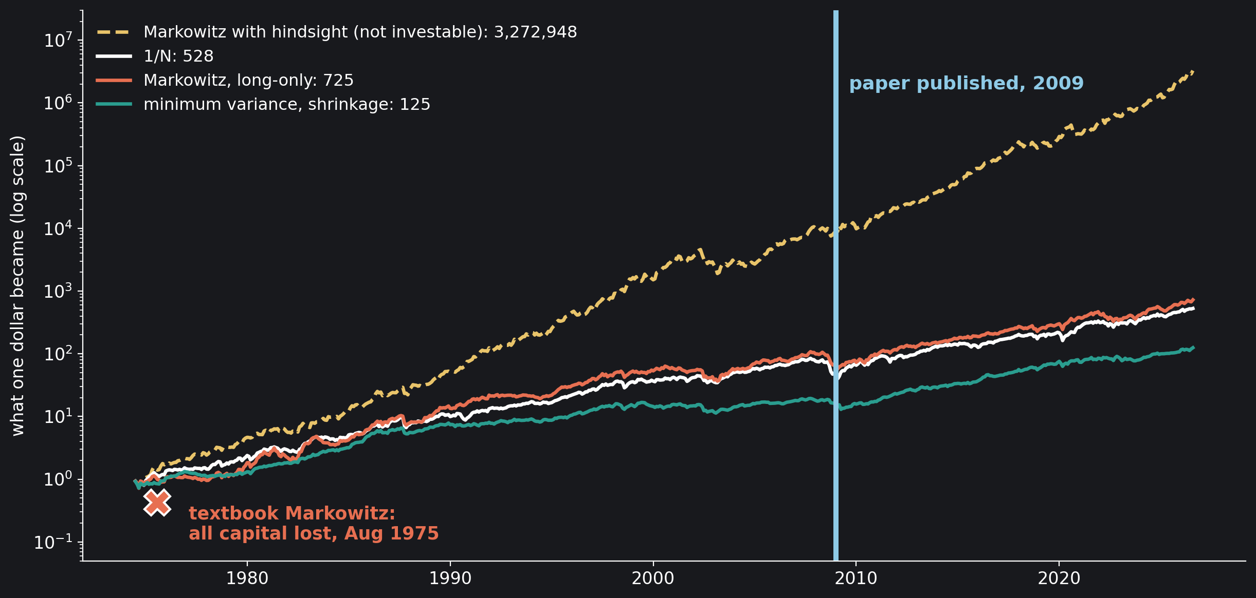
Over the 52 years from 1974, 1/N’s Sharpe ratio is 0.55. Long-only Markowitz draws level at 0.54, long-only minimum variance edges ahead at 0.59, and shrinkage minimum variance trails at 0.47. Long-only Markowitz ends with more dollars than 1/N, 725 against 528, by taking more risk for a little less return per unit of it. The textbook rule has a negative Sharpe ratio even as a series of returns, −0.10, and as an investment it is over in August 1975, in its fourteenth month. As a series it goes on, and in January 1981 a single month’s return is −13,498%. Hindsight Markowitz doubles 1/N, 1.17, and turns a dollar into 3.3 million against 1/N’s 528.
After the paper, from January 2009, the repaired versions edge ahead of 1/N’s 0.80: long-only Markowitz 0.85, shrinkage minimum variance 0.90, long-only minimum variance 0.87. That margin is small, it is one stretch of seventeen years, and it ignores the trading those rules do; the textbook rule, starting afresh with a dollar in 2009, is wiped out by January 2010. A ten-year window, 120 months, tells the same story in both periods (the last two lines of the output). Figure 2 shows the dollars.
How Long Is Long Enough
Raymond Kan and Guofu Zhou worked out in 2007 what the textbook rule earns on average when its inputs are estimated. Take an investor who values a portfolio $w$ of excess returns at $U(w) = w^\top\mu – \tfrac{\gamma}{2}\,w^\top\Sigma w$, with $\gamma$ his aversion to risk. Knowing the true $\mu$ and $\Sigma$ of $N$ assets, he would hold $w^* = \Sigma^{-1}\mu/\gamma$ and earn $\theta^2/(2\gamma)$, where $\theta^2 = \mu^\top\Sigma^{-1}\mu$ is the squared Sharpe ratio of the best mix. Estimating both from $T$ months of normal returns, with the sample mean $\hat\mu$ and the maximum-likelihood covariance $\hat\Sigma$, he holds $\hat w = \hat\Sigma^{-1}\hat\mu/\gamma$ and earns on average
DeMiguel, Garlappi and Uppal set this against 1/N, held in the amount that suits the same investor best, which earns $S_{ew}^2/(2\gamma)$, with $S_{ew}$ the Sharpe ratio of 1/N. The risk aversion cancels, and the textbook rule beats 1/N on average only when (their Proposition 1)
With many months, $k \to 1$ and $h \to 0$ and the rule earns the whole $\theta^2$; with few, $k$ falls below one and $h$, which grows with the number of assets, eats the rest. To use it, $\theta^2$ and $S_{ew}^2$ come from the 48 industries’ whole 57 years. The sample $\hat\theta^2$ is flattered by the same noise as everything else, so it is replaced by Kan and Zhou’s unbiased estimator, $\big((T-N-2)\,\hat\theta^2 – N\big)/T$.
How Long Is Long Enough
from scipy.optimize import brentq

E = X - rf_i[:, None]                  # 686 months, 48 industries
T0, N = E.shape
mu, S, one = E.mean(0), np.cov(E.T, bias=True), np.ones(N)
th2_hat = mu @ np.linalg.solve(S, mu)
th2 = ((T0 - N - 2) * th2_hat - N) / T0     # Kan and Zhou's unbiased
sew2 = (one @ mu) ** 2 / (one @ S @ one)
for name, x in (("sample", th2_hat), ("unbiased", th2), ("1/N", sew2)):
    print(f"{name:>9} Sharpe ratio: {np.sqrt(12 * x):.2f} a year")

#    sample Sharpe ratio: 1.21 a year
#  unbiased Sharpe ratio: 0.72 a year
#       1/N Sharpe ratio: 0.46 a year
The industries’ sample $\hat\theta$, 1.21 a year, is the Sharpe ratio the hindsight portfolio shows on the 57 years it was fitted to. Unbiased, it is 0.72, against 1/N’s 0.46: the best mix is better than 1/N, but by less than hindsight suggests. The critical window is where the textbook rule’s expected utility reaches 1/N’s.
The Critical Window
def plug_in(T, N, th2):                # 2 gamma E[U] of the textbook rule
    k = T / (T - N - 2) * (2 - T * (T - 2) / ((T - N - 1) * (T - N - 4)))
    h = N * T * (T - 2) / ((T - N - 1) * (T - N - 2) * (T - N - 4))
    return k * th2 - h

def critical_T(N, th2, sew2):          # months for it to beat 1/N
    return brentq(lambda T: plug_in(T, N, th2) - sew2, N + 4.001, 1e7)

for n in (48, 25):
    t = critical_T(n, th2, sew2)
    print(f"{n} assets: {t:,.0f} months = {t / 12:,.0f} years")
print("the paper's calibration, Sharpe ratios 0.15 and 0.12 a month:")
for n in (25, 50):
    print(f"{n} assets: {critical_T(n, 0.15**2, 0.12**2):,.0f} months")

# 48 assets: 2,054 months = 171 years
# 25 assets: 1,073 months = 89 years
# the paper's calibration, Sharpe ratios 0.15 and 0.12 a month:
# 25 assets: 3,239 months
# 50 assets: 6,469 months
With the unbiased $\theta^2$ and 1/N’s $S_{ew}^2$, the textbook rule on 48 industries needs 2,054 months, 171 years of data, before it beats 1/N on average; on 25 assets with the same two Sharpe ratios, 1,073 months, 89 years. Fed the paper’s own calibration for the US stock market, a monthly $S^* = 0.15$ against $S_{ew} = 0.12$, the same formula returns 3,239 months for 25 assets and 6,469 for 50, the paper’s “around 3000” and “about 6000”.
Two Ways
The closed form assumes normal returns and nothing else, so a simulation can test it. The simulated market has the industries’ covariance matrix and means rescaled to the two calibrated numbers: the part of $\mu$ that 1/N captures, a multiple of $\Sigma\mathbf{1}$, is kept, and the rest is shrunk until $\mu^\top\Sigma^{-1}\mu$ equals the unbiased $\theta^2$. Each draw is a window of $T$ months of normal returns, the textbook rule fitted to it, and the rule’s true utility; the table shows the average as a share of the true optimum’s.
Two Ways
a = (one @ mu) / (one @ S @ one)       # the 1/N part of the means ...
rest = mu - a * S @ one                # ... and the rest: 1'rest = 0
c = np.sqrt((th2 - sew2) / (rest @ np.linalg.solve(S, rest)))
mu_c = a * S @ one + c * rest          # theta^2 = th2, S_ew^2 = sew2
L = np.linalg.cholesky(S)
rng = np.random.default_rng(20261011)
print(f"{'window':>13}{'Monte Carlo':>17}{'closed form':>13}{'gap / s.e.':>12}")
mc = {}
for T, n in ((120, 2000), (1200, 400), (2400, 400), (4800, 400),
             (9600, 200)):
    u = np.empty(n)
    for i in range(n):
        Z = rng.standard_normal((T, N)) @ L.T + mu_c   # T normal months
        w = np.linalg.solve(np.cov(Z.T, bias=True), Z.mean(0))
        u[i] = (2 * w @ mu_c - w @ S @ w) / th2       # gamma = 1
    mc[T] = u.mean(), u.std(ddof=1) / np.sqrt(n)
    cf = plug_in(T, N, th2) / th2
    print(f"{T:>6} months{mc[T][0]:>10.3f} ± {mc[T][1]:.3f}{cf:>13.3f}"
          f"{(mc[T][0] - cf) / mc[T][1]:>12.2f}")

#        window      Monte Carlo  closed form  gap / s.e.
#    120 months   -47.925 ± 0.485      -47.594       -0.68
#   1200 months    -0.090 ± 0.012       -0.087       -0.30
#   2400 months     0.490 ± 0.005        0.491       -0.08
#   4800 months     0.757 ± 0.003        0.753        1.42
#   9600 months     0.881 ± 0.002        0.879        1.36
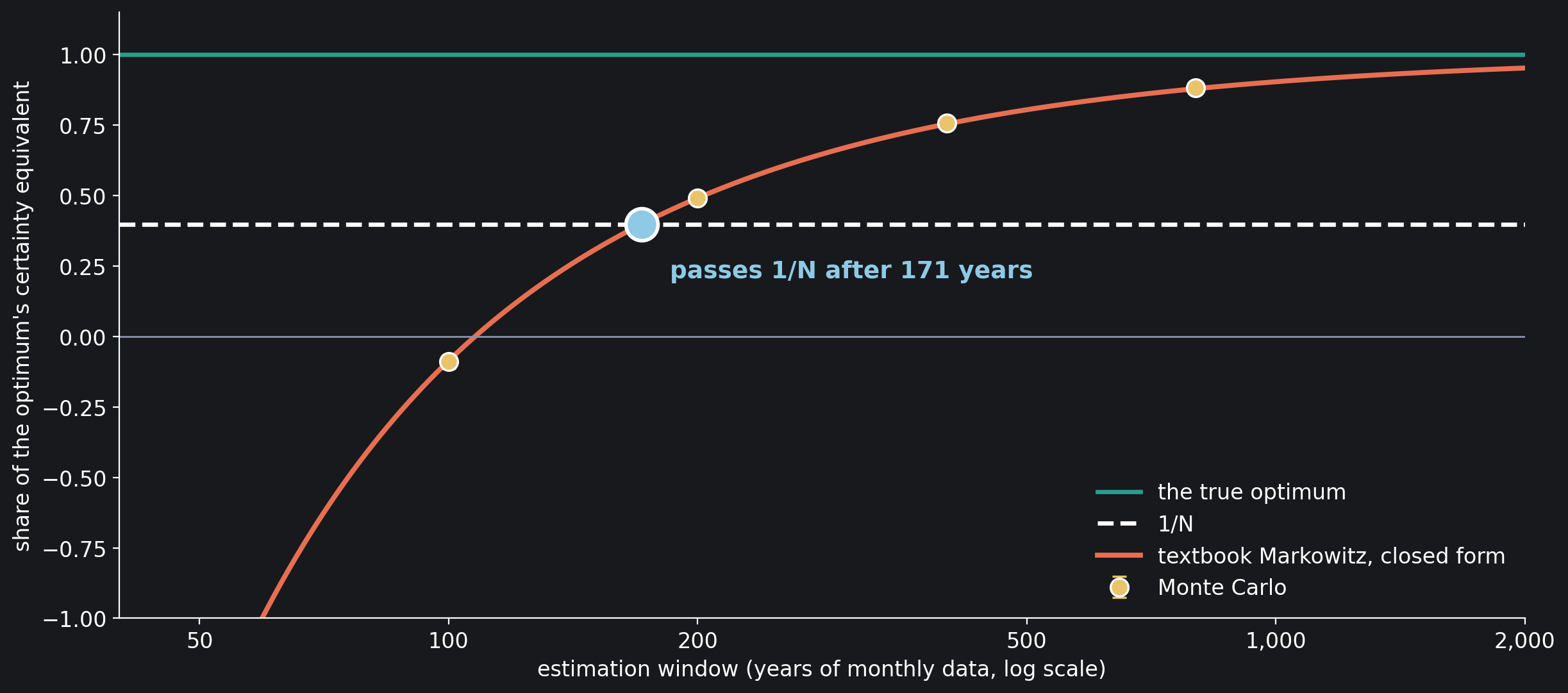
The simulation and the formula agree at every window, each time within one and a half standard errors of the simulation. With ten years of data, the longer of the two windows the paper calls typical, the textbook rule’s expected certainty equivalent is minus 48 times the optimum’s: on average the investor would do better in T-bills. At a hundred years it is still below zero, at two hundred it has reached half of the optimum, and 1/N, which captures 40% of the optimum without estimating anything, is passed only at 171 years. Figure 3 draws the curve.
Your Own Portfolio
The stock study runs again from the cell below with your own numbers: the stocks in each random portfolio and the trading days behind each estimate (more than the number of stocks; the file holds 1,258 days, and a longer window leaves fewer to test on). It takes about half a minute for 25 stocks, twice that for 50. A two-year window, `WINDOW_DAYS = 500`, lifts long-only Markowitz to a win over 1/N in 38.3% of portfolios but drops the minimum-variance rules to 28.9% and 24.1%, over a shorter test that starts in February 2015; 50 stocks with a one-year window give long-only Markowitz 17.2%.
Your Own Portfolio
N_STOCKS = 25          # stocks in each random portfolio
WINDOW_DAYS = 250      # trading days behind each estimate (a year = 252)

scoreboard(stocks_study(N_STOCKS, WINDOW_DAYS))

#                            median  1 became   wiped   beats   traded
#                            Sharpe  (median)     out     1/N  a month
# 1/N                          0.89      1.56    0.0%               4%
# Markowitz, textbook         wiped      0.00   86.2%    1.7%   1,098%
# Markowitz, long-only         0.59      1.40    0.0%   14.9%      58%
# Min variance, shrinkage      0.85      1.45    0.0%   44.5%      32%
# Min variance, long-only      0.82      1.42    0.0%   39.2%      22%
# Markowitz, hindsight         2.28      8.90    0.0%  100.0%      34%
What the Numbers Show
The formula is not wrong. Fed the whole sample’s own means and covariances, it more than doubles 1/N’s Sharpe ratio, on the stocks and over the industries’ 52 years, and even with the in-sample flattery removed the closed form puts the best mix of the 48 industries at a Sharpe ratio of 0.72 against 1/N’s 0.46. What fails is the estimate of the means. Every strategy here that uses them lost to 1/N on the stocks: the textbook rule was wiped out in 862 portfolios of 1,000, and its long-only version beat 1/N in 149. Throw the means away and keep the covariances, which a year of daily data measures well, and the minimum-variance rules come close to 1/N, winning 445 and 392 times in 1,000 with median Sharpe ratios of 0.85 and 0.82 against 0.89. On the industries, with dividends, the repaired versions sit between 0.47 and 0.59 around 1/N’s 0.55 over 52 years, and in the seventeen years after the paper they edge ahead, by a small margin, over one stretch of history.
The closed form says why, and how far away the cure is: with the industries’ own numbers, 171 years of monthly data before the textbook rule beats 1/N on average. The Talmud’s rule needs no estimate at all. Markowitz’s 50/50 split of 1952 was the same rule, with N = 2.
Sources
- Babylonian Talmud, Bava Metzia 42a, in the William Davidson Edition on Sefaria: English from the Koren Noé Talmud, with commentary by Rabbi Adin Even-Israel Steinsaltz (CC BY-NC); the bracketed words are the commentary’s.
- H. Markowitz, “Portfolio Selection”, Journal of Finance 7 (1952) 77–91, doi:10.1111/j.1540-6261.1952.tb01525.x.
- The Sveriges Riksbank Prize in Economic Sciences in Memory of Alfred Nobel 1990, nobelprize.org.
- J. Zweig, “What Harry Markowitz Meant”, jasonzweig.com: the 1997 interview and Markowitz’s 2009 clarification.
- V. DeMiguel, L. Garlappi and R. Uppal, “Optimal Versus Naive Diversification: How Inefficient is the 1/N Portfolio Strategy?”, Review of Financial Studies 22 (2009) 1915–1953, doi:10.1093/rfs/hhm075.
- J. Tu and G. Zhou, “Markowitz meets Talmud: A combination of sophisticated and naive diversification strategies”, Journal of Financial Economics 99 (2011) 204–215, doi:10.1016/j.jfineco.2010.08.013.
- R. Kan and G. Zhou, “Optimal Portfolio Choice with Parameter Uncertainty”, Journal of Financial and Quantitative Analysis 42 (2007) 621–656, doi:10.1017/S0022109000004129.
- O. Ledoit and M. Wolf, “A well-conditioned estimator for large-dimensional covariance matrices”, Journal of Multivariate Analysis 88 (2004) 365–411, doi:10.1016/S0047-259X(03)00096-4.
- C. Nugent, “S&P 500 stock data”, Kaggle dataset camnugent/sandp500 (CC0), daily closes from 8 February 2013 to 7 February 2018.
- K. R. French, Data Library: 48 Industry Portfolios and the Fama/French 3 Factors (the one-month T-bill rate), built from the CRSP database of August 2026, mba.tuck.dartmouth.edu.
- S&P 500 dividend yield at the end of each year, multpl.com: between 1.84% and 2.11% for 2013 to 2017.
Every number in this notebook is computed by its own cells from the two data files.
Working on a pricing model or risk system? Let’s talk.