
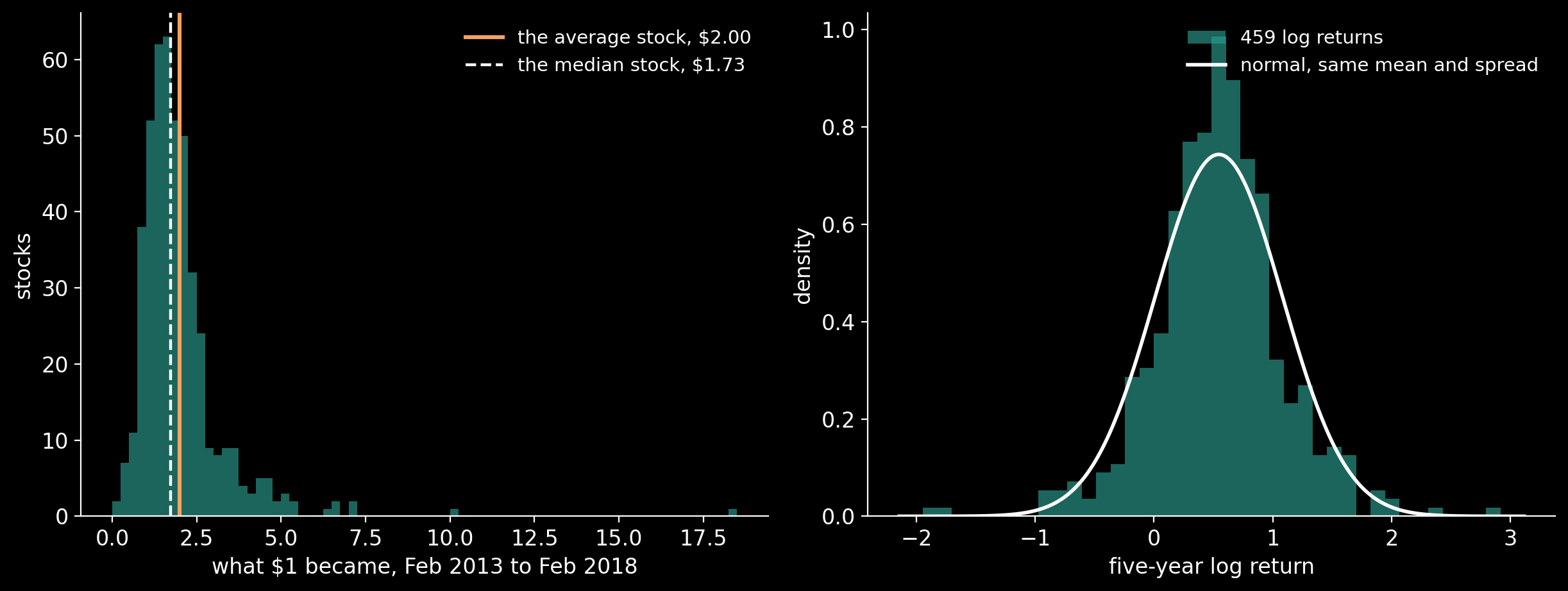
Put a dollar into each of 459 S&P 500 stocks in February 2013 and hold every one of them for five years. The average stock, which is what all 459 dollars together returned, turned $1 into $2.00. The median stock turned it into $1.73, and 288 of the 459, 62.7%, finished below the average.
Nothing was wrong with those 288 stocks in particular. Compounding puts most stocks below their own average, by an amount a one-line formula predicts: 60.6% here, against the 62.7% that happened. This notebook measures the gap, shows why it widens the longer a stock is held, splits it stock by stock into volatility drag, and finds where the five years’ gains went.
Five Years of 459 Stocks
The returns are daily closing prices of the S&P 500 members from 8 February 2013 to 7 February 2018, from a public-domain Kaggle dataset: 470 stocks have a price on every one of the 1,259 days. The prices are not adjusted for splits and spin-offs, so a stock is dropped if it has a one-day move by a factor of more than 1.75, or a move of more than 20% that reverses by more than 20% the next day, which is a bad print; that removes 11 and leaves 459. These are price returns, without dividends, and the 459 are survivors: every stock here was still trading in February 2018.
Five Years of 459 Stocks
import numpy as np
import pandas as pd

rets = pd.read_csv("data/sp500_returns.csv", index_col="date", parse_dates=True)
X = rets.sum()                        # each stock's five-year log return
W = np.exp(X)                         # $1 in each stock, bought and held
print(f"{rets.shape[1]} stocks, {rets.shape[0]} trading days, "
      f"{rets.index[0]:%d %b %Y} to {rets.index[-1]:%d %b %Y}")
print(f"$1 in the average stock:  ${W.mean():.2f}")
print(f"$1 in the median stock:   ${W.median():.2f}")
print(f"stocks below the average: {np.sum(W < W.mean())} of {W.size} "
      f"({np.mean(W < W.mean()):.1%})")

# 459 stocks, 1258 trading days, 11 Feb 2013 to 07 Feb 2018
# $1 in the average stock:  $2.00
# $1 in the median stock:   $1.73
# stocks below the average: 288 of 459 (62.7%)
Why the Average Beats the Median
Write a stock’s final wealth as $W = e^{X}$, where $X$ is its log return over the five years. If $X$ is normal across the stocks, with mean $m$ and spread $s$, the average stock ends with $e^{m + s^2/2}$ and the median stock with $e^{m}$. A stock beats the average only if its log return clears $m + s^2/2$, which is half a standard deviation above the middle:
Normality is not what makes it true. For any spread of $X$ that is symmetric about its median, Jensen’s inequality puts the average of $e^{X}$ above $e$ raised to that median, which is the median stock’s wealth, so at least half the stocks sit below the average whenever they differ at all. The normal case only says how far below.
The Lognormal Prediction
from scipy.stats import norm, skew, kurtosis

s = X.std(ddof=1)
print(f"spread of the five-year log returns, s: {s:.3f}")
print(f"predicted share below the average, Phi(s/2): {norm.cdf(s / 2):.1%}")
print(f"skew of the log returns: {skew(X):.2f}, "
      f"excess kurtosis: {kurtosis(X):.2f}")
print(f"skew of the wealth itself: {skew(W):.2f}")

# spread of the five-year log returns, s: 0.536
# predicted share below the average, Phi(s/2): 60.6%
# skew of the log returns: -0.12, excess kurtosis: 2.34
# skew of the wealth itself: 5.11
The spread of the five-year log returns is 0.536, so the formula predicts 60.6% below the average; 62.7% were. The log returns are close to symmetric, with a skew of −0.12, but fatter-tailed than a normal curve, with an excess kurtosis of 2.34. The wealth they compound into is not symmetric at all: its skew is 5.11, a long tail of stocks that multiplied several times over.
The Longer You Hold
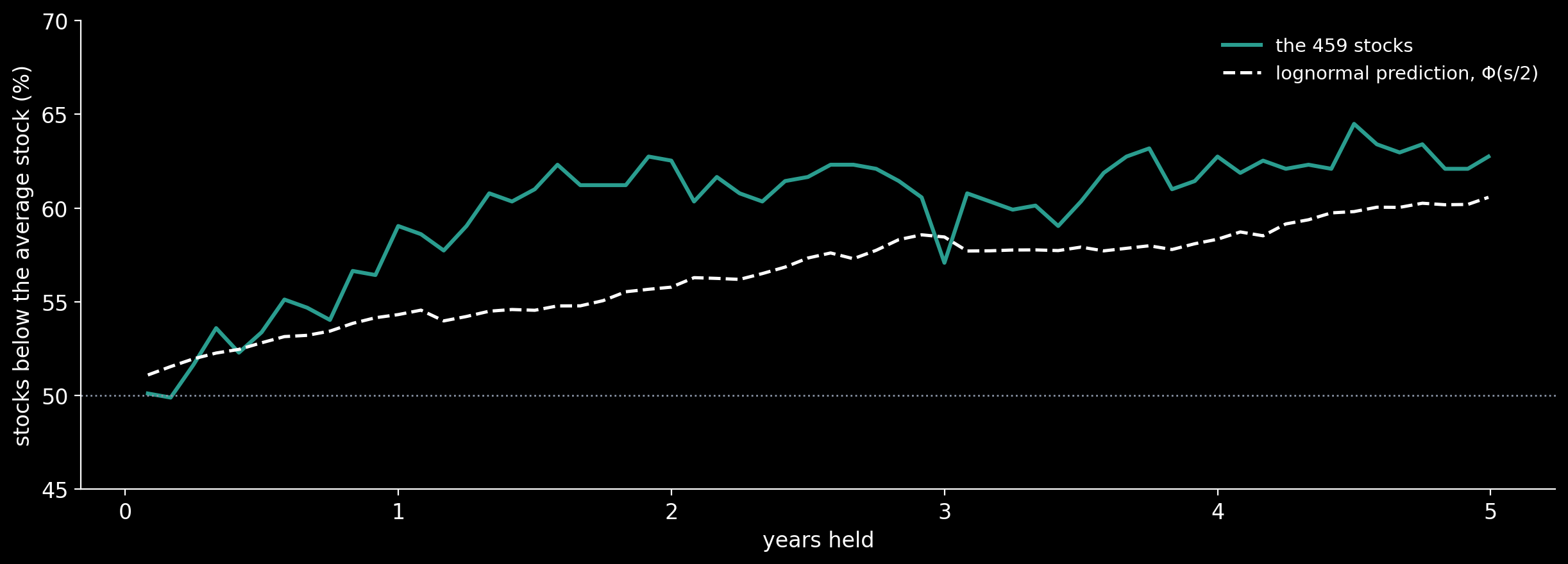
The spread $s$ of the log returns grows with the time a stock is held, roughly as its square root, so $\Phi(s/2)$ grows too. Year by year the share below the average stays just above half, as low as 50.3% in 2015, 231 of the 459 stocks:
Year by Year
print("year   days   below the average   Phi(s/2)")
for year, g in rets.groupby(rets.index.year):
    if len(g) < 200:                  # 2018 holds only five weeks
        continue
    w = np.exp(g.sum())
    pred = norm.cdf(np.log(w).std() / 2)
    print(f"{year}   {len(g):4d}   {np.mean(w < w.mean()):17.1%}   {pred:8.1%}")

# year   days   below the average   Phi(s/2)
# 2013    225               55.3%      54.0%
# 2014    252               51.0%      53.7%
# 2015    252               50.3%      55.1%
# 2016    252               52.1%      54.1%
# 2017    251               54.7%      54.5%
The Longer You Hold
cum = rets.cumsum()
ends = np.append(np.arange(21, len(rets), 21), len(rets))   # a month at a time
H = ends / 252                            # years held
wealth = [np.exp(cum.iloc[k - 1]) for k in ends]   # a dollar, by horizon
share = np.array([np.mean(w < w.mean()) for w in wealth])
pred = np.array([norm.cdf(cum.iloc[k - 1].std() / 2) for k in ends])
for yrs in (0.5, 1, 2, 3, 4, 5):
    i = np.argmin(np.abs(H - yrs))
    print(f"held {H[i]:3.1f} years: {share[i]:.1%} below the average "
          f"(Phi(s/2): {pred[i]:.1%})")

# held 0.5 years: 53.4% below the average (Phi(s/2): 52.8%)
# held 1.0 years: 59.0% below the average (Phi(s/2): 54.3%)
# held 2.0 years: 62.5% below the average (Phi(s/2): 55.8%)
# held 3.0 years: 57.1% below the average (Phi(s/2): 58.5%)
# held 4.0 years: 62.7% below the average (Phi(s/2): 58.3%)
# held 5.0 years: 62.7% below the average (Phi(s/2): 60.6%)
Held from February 2013, the share rises from 53.4% at six months to 59.0% at one year and 62.7% at five, though not smoothly: at three years it was back to 57.1%. The prediction rises more smoothly, from 52.8% to 60.6%. Over one year, “most” is barely true; over five, it is almost two in three.
Volatility Drag, Stock by Stock
The same inequality works inside each stock. A stock’s growth rate is its average daily return less about half its daily variance, $g \approx \mu – \tfrac{1}{2}\sigma^2$, so of two stocks with the same average return, the more volatile one ends with less.
Volatility Drag, Stock by Stock
simple = np.expm1(rets)                   # daily simple returns
mu, var = simple.mean(), simple.var()
g = rets.mean()                           # the growth rate actually achieved
drag = 252 * (mu - g)                     # the yearly gap between the two
print(f"median yearly arithmetic return: {252 * mu.median():.1%}")
print(f"median yearly growth rate:       {252 * g.median():.1%}")
print(f"median yearly drag, mean minus growth: {drag.median():.2%}")
print(f"half the variance predicts:            {(252 * var / 2).median():.2%}")
r = np.corrcoef(drag, var)[0, 1]
print(f"correlation of the two, stock by stock: {r:.4f}")

# median yearly arithmetic return: 13.6%
# median yearly growth rate:       11.0%
# median yearly drag, mean minus growth: 2.56%
# half the variance predicts:            2.56%
# correlation of the two, stock by stock: 0.9992
For the median stock, an average return of 13.6% a year compounded at 11.0%. The drag between them, 2.56% a year, matches half the variance to the hundredth of a percent, and across the 459 stocks the two agree with a correlation of 0.9992.
Where the Gains Came From
A long right tail means a few stocks carried the average.
Where the Gains Came From
gain = (W - 1).sort_values(ascending=False)
top = int(round(0.1 * gain.size))
print(f"$1 in each of {gain.size} stocks gained ${gain.sum():.0f} in all")
print(f"the top {top} stocks made {gain.iloc[:top].sum() / gain.sum():.0%} "
      f"of it")
print(f"the top half made {gain.iloc[:gain.size // 2].sum() / gain.sum():.0%}")
print(f"stocks that lost money: {np.sum(W < 1)}")

# $1 in each of 459 stocks gained $460 in all
# the top 46 stocks made 39% of it
# the top half made 89%
# stocks that lost money: 58
Together the 459 dollars gained $460. The best 46 stocks, a tenth of them, made 39% of that gain, and the best half made 89% of it. Fifty-eight stocks lost money outright.
Compounding Alone
Keep each stock’s own drift and volatility, but let the stocks move independently of each other, and simulate the five years 200 times.
Compounding Alone
rng = np.random.default_rng(20261005)
m, sd, T = rets.mean().to_numpy(), rets.std().to_numpy(), len(rets)
X_sim = rng.normal(m * T, sd * np.sqrt(T), size=(200, m.size))   # 200 markets
sims = np.array([np.mean(np.exp(x) < np.exp(x).mean()) for x in X_sim])
print(f"independent stocks, same drifts and vols: {sims.mean():.1%} below "
      f"(middle 90%: {np.quantile(sims, 0.05):.1%} "
      f"to {np.quantile(sims, 0.95):.1%})")
x_sim = rng.normal(m * T, sd * np.sqrt(T))
print(f"their spread s: {x_sim.std():.3f}, against the market's {s:.3f}")
print(f"the real market: {np.mean(W < W.mean()):.1%} below")

# independent stocks, same drifts and vols: 67.9% below (middle 90%: 64.0% to 72.6%)
# their spread s: 0.780, against the market's 0.536
# the real market: 62.7% below
Independent stocks would leave 67.9% below the average, more than the real 62.7%. The reason is the market itself. It moves every stock together, so it is part of each stock’s volatility but spreads no stock away from the others: independent stocks with the same volatilities would spread out to 0.780, against the 0.536 the real 459 reached.
What It Means
The average stock is not a stock. It is a portfolio of all 459, and it collects the mean of their outcomes, while one stock picked at random most likely ends up near the median. The gap between the two is volatility, compounded: small over a year, and almost two stocks in three over five.
These 459 are survivors. Stocks that left the index or stopped trading during the five years, often after large losses, are not in the data, so the true share below the average is likely higher. Over the whole US market since 1926, Bessembinder (2018) found that most common stocks did worse over their lifetimes than one-month Treasury bills, and that a small fraction of companies accounts for all of the market’s net wealth creation.
Sources
- H. Bessembinder, “Do stocks outperform Treasury bills?”, Journal of Financial Economics 129 (2018) 440–457.
- C. Nugent, “S&P 500 stock data”, Kaggle dataset camnugent/sandp500 (CC0: Public Domain).
Working on a pricing model or risk system? Let’s talk.