
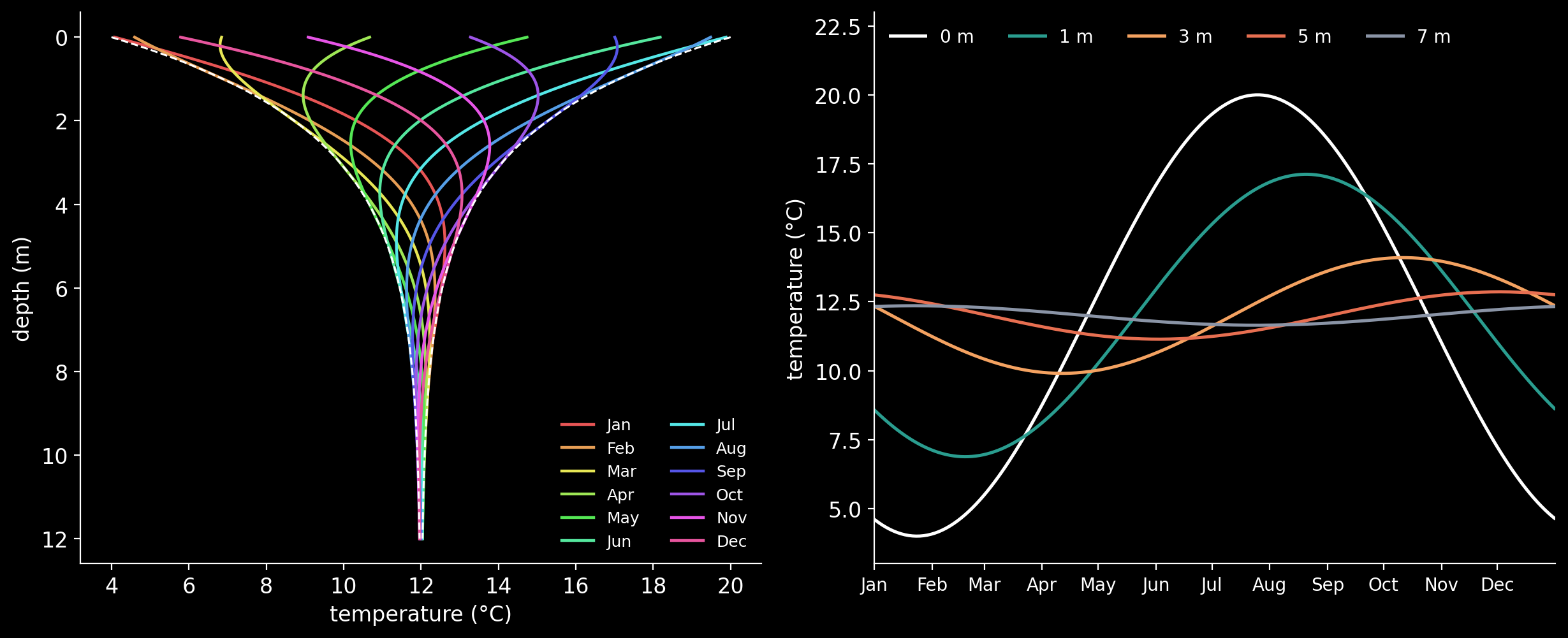
Dig into the ground in July and it gets cooler with every spadeful; dig in January and it gets warmer. Go deeper and the seasons arrive late: a few metres down the summer comes in autumn, and at about seven metres in ordinary soil the calendar is turned over, so the ground is at its warmest in January and its coldest in July. Fourier, who built the theory of heat between 1807 and 1822, solved this very problem in 1809 and later stated its rule plainly in a memoir on the temperatures of the Earth: the depth the variations reach is exactly proportional to the square root of their period, which is why the daily swing goes only a nineteenth as deep as the yearly one.
This notebook writes down the exact solution, solves the same equation on a grid and checks the two against each other, draws the calendar of the ground metre by metre, and then runs the problem backwards the way William Thomson, later Lord Kelvin, did in a paper of 1861: from two buried thermometers, it reads off how fast heat spreads through the soil.
The Exact Wave
Heat in the ground obeys the heat equation, $\partial T/\partial t = \kappa\, \partial^2 T/\partial z^2$, with depth $z$ measured downwards and $\kappa$ the soil’s thermal diffusivity. If the surface swings once a year around its mean, $T(0,t) = \bar T + A\cos\omega(t – t_{\max})$ with $\omega = 2\pi/\text{year}$, the swing that settles in below is
Every metre down, the swing shrinks by the same factor and runs later by the same number of days. The damping depth $d$ sets both: the swing falls by a factor $e$ over each $d$, and at $z = \pi d$ the wave is half a year late.
The numbers below are assumptions, stated once: an idealised temperate site with an annual mean of 12 °C at the surface, a swing of ±8 °C, the warmest day on 25 July, and $\kappa = 5 \times 10^{-7}$ m²/s, a typical value for damp soil. Measured diffusivities for soils run from about $2 \times 10^{-7}$ to above $10^{-6}$ m²/s, mostly according to how wet the soil is.
The Wave, Metre by Metre
import numpy as np
from datetime import date, timedelta

YEAR = 365.25                          # days
kappa = 5e-7 * 86400                   # m²/day: 5e-7 m²/s, damp soil
omega = 2 * np.pi / YEAR               # per day
d = np.sqrt(2 * kappa / omega)         # the damping depth, metres
Tbar, A = 12.0, 8.0                    # yearly mean and swing at the surface, °C
t_max = 205.5                          # day 0 = 1 January; 205.5 = noon on 25 July

def exact(z, t):
    return Tbar + A * np.exp(-z / d) * np.cos(omega * (t - t_max) - z / d)

def calendar(day):
    day = int(np.floor(day % YEAR)) % 365     # day 0 runs through 1 January
    when = date(2025, 1, 1) + timedelta(days=day)
    return f"{when.day} {when.strftime('%b')}"

print(f"damping depth d = {d:.3f} m")
print(f"half a year late at pi*d = {np.pi * d:.2f} m")
print(f"each metre: swing x {np.exp(-1 / d):.3f}, {1 / d / omega:.1f} days later")
print()
print(" depth   swing     late by   warmest")
for z in (0, 1, 2, 3, 5, 7, 10):
    lag = z / d / omega
    swing = A * np.exp(-z / d)
    print(f"{z:4d} m  ±{swing:5.2f} °C  {lag:5.1f} days  {calendar(t_max + lag)}")

# damping depth d = 2.241 m
# half a year late at pi*d = 7.04 m
# each metre: swing x 0.640, 25.9 days later
#
#  depth   swing     late by   warmest
#    0 m  ± 8.00 °C    0.0 days  25 Jul
#    1 m  ± 5.12 °C   25.9 days  20 Aug
#    2 m  ± 3.28 °C   51.9 days  15 Sep
#    3 m  ± 2.10 °C   77.8 days  11 Oct
#    5 m  ± 0.86 °C  129.7 days  2 Dec
#    7 m  ± 0.35 °C  181.6 days  22 Jan
#   10 m  ± 0.09 °C  259.4 days  10 Apr
The Same Equation on a Grid
The exact formula holds for ground that goes down forever and has swung for ever. A grid solver makes neither promise, so it is the honest check. The column is 30 metres deep, about thirteen damping depths, cut into thin layers, and stepped through time with the Crank–Nicolson scheme (1947), which averages the flow of heat at the start and the end of each step and is second-order accurate in both space and time. It starts on 1 January from the exact profile, runs for two years, and is compared with the formula on the last day. The bottom of the column is held to the formula too, so that the only error left is the grid’s own.
Second order means that halving both the layer and the step should cut the error by four.
Crank–Nicolson Against the Exact Wave
from scipy.linalg import solve_banded

def crank_nicolson(L, nz, dt, t0, t1, T_start, top, bottom, keep=False):
    z = np.linspace(0, L, nz + 1)
    r = kappa * dt / (z[1] - z[0]) ** 2
    band = np.zeros((3, nz - 1))
    band[0, 1:], band[1], band[2, :-1] = -r / 2, 1 + r, -r / 2
    T, t, kept = T_start(z).copy(), t0, []
    for _ in range(int(round((t1 - t0) / dt))):
        t += dt
        rhs = (1 - r) * T[1:-1] + r / 2 * (T[:-2] + T[2:])
        rhs[0] += r / 2 * top(t)
        rhs[-1] += r / 2 * bottom(t)
        T[1:-1] = solve_banded((1, 1), band, rhs, check_finite=False)
        T[0], T[-1] = top(t), bottom(t)
        if keep:
            kept.append(T.copy())
    return z, T, t, np.array(kept)

L, err = 30.0, []
print(" layer    step     largest error vs the formula")
for nz, dt in ((150, 4.0), (300, 2.0), (600, 1.0), (1200, 0.5)):
    z, T, t, _ = crank_nicolson(L, nz, dt, 0.0, 2 * YEAR, lambda z: exact(z, 0.0),
                                lambda t: exact(0.0, t), lambda t: exact(L, t))
    err.append(np.max(np.abs(T - exact(z, t))))
    tail = f"   {err[-2] / err[-1]:.2f} x smaller" if len(err) > 1 else ""
    print(f"{100 * L / nz:4.1f} cm  {dt:4.1f} days  {err[-1]:.2e} °C{tail}")
print(f"observed order of accuracy: {np.log2(err[-2] / err[-1]):.3f}")

#  layer    step     largest error vs the formula
# 20.0 cm   4.0 days  1.92e-03 °C
# 10.0 cm   2.0 days  4.88e-04 °C   3.93 x smaller
#  5.0 cm   1.0 days  1.22e-04 °C   4.00 x smaller
#  2.5 cm   0.5 days  3.04e-05 °C   4.02 x smaller
# observed order of accuracy: 2.006
The Calendar of the Ground
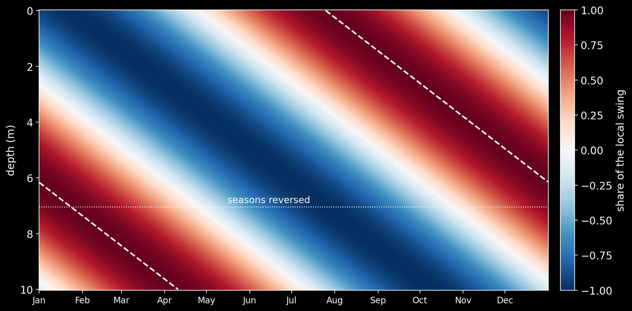
Read the grid’s year depth by depth, one profile at noon each day, and the seasons slide down the calendar. The table takes each depth’s warmest and coldest day straight from the daily solution, with no formula in between, and then compares a cellar three metres down with the surface in midwinter and midsummer.
Warmest and Coldest, Depth by Depth
dz = z[1] - z[0]
print(" depth   swing     warmest   coldest")
for depth in (0, 1, 2, 3, 5, 7, 10):
    i = int(round(depth / dz))
    s = year2[:, i]
    hot, cold = calendar(d2[s.argmax()]), calendar(d2[s.argmin()])
    print(f"{depth:4d} m  ±{(s.max() - s.min()) / 2:5.2f} °C  {hot:>7}   {cold:>7}")
print()
i3 = int(round(3 / dz))
for label, day in (("15 January", 14.5), ("15 July", 195.5)):
    k = np.argmin(np.abs(doy - day))
    top, cellar = year2[k, 0], year2[k, i3]
    print(f"{label:10s}: surface {top:5.2f} °C, cellar at 3 m {cellar:5.2f} °C")

#  depth   swing     warmest   coldest
#    0 m  ± 8.00 °C   25 Jul    23 Jan
#    1 m  ± 5.12 °C   20 Aug    18 Feb
#    2 m  ± 3.28 °C   15 Sep    16 Mar
#    3 m  ± 2.10 °C   11 Oct    11 Apr
#    5 m  ± 0.86 °C    2 Dec     2 Jun
#    7 m  ± 0.35 °C   22 Jan    24 Jul
#   10 m  ± 0.09 °C   10 Apr    10 Oct
#
# 15 January: surface  4.08 °C, cellar at 3 m 11.82 °C
# 15 July   : surface 19.88 °C, cellar at 3 m 12.13 °C
A Day Against a Year
The same formula holds for the daily swing, with the period of one day in place of a year. The damping depth goes as the square root of the period, so the daily wave dies $\sqrt{365.25}$ times closer to the surface. Fourier gave the number as nineteen.
Nineteen Times Shallower
d_day = np.sqrt(2 * kappa / (2 * np.pi / 1.0))   # damping depth of the daily wave
fade = np.log(100)                               # where 1% of the swing is left
print(f"damping depth, daily wave:  {100 * d_day:.1f} cm")
print(f"damping depth, yearly wave: {d:.2f} m")
print(f"1% of the daily swing left at  {100 * fade * d_day:.0f} cm")
print(f"1% of the yearly swing left at {fade * d:.1f} m")
print(f"ratio: {d / d_day:.2f}   sqrt(365.25) = {np.sqrt(YEAR):.2f}")

# damping depth, daily wave:  11.7 cm
# damping depth, yearly wave: 2.24 m
# 1% of the daily swing left at  54 cm
# 1% of the yearly swing left at 10.3 m
# ratio: 19.11   sqrt(365.25) = 19.11
Reading the Soil From Two Thermometers
James David Forbes buried thermometers at several depths at three sites near Edinburgh, in the trap rock of Calton Hill, the sand of the Experimental Garden and the sandstone of Craigleith Quarry; the Calton Hill readings began in 1837. In a paper of 1861, William Thomson took their readings and ran the problem backwards. The formula says the yearly wave shrinks by $e^{-\Delta z/d}$ and runs late by $\Delta z/d$ radians between two depths $\Delta z$ apart, so either measurement gives the diffusivity:
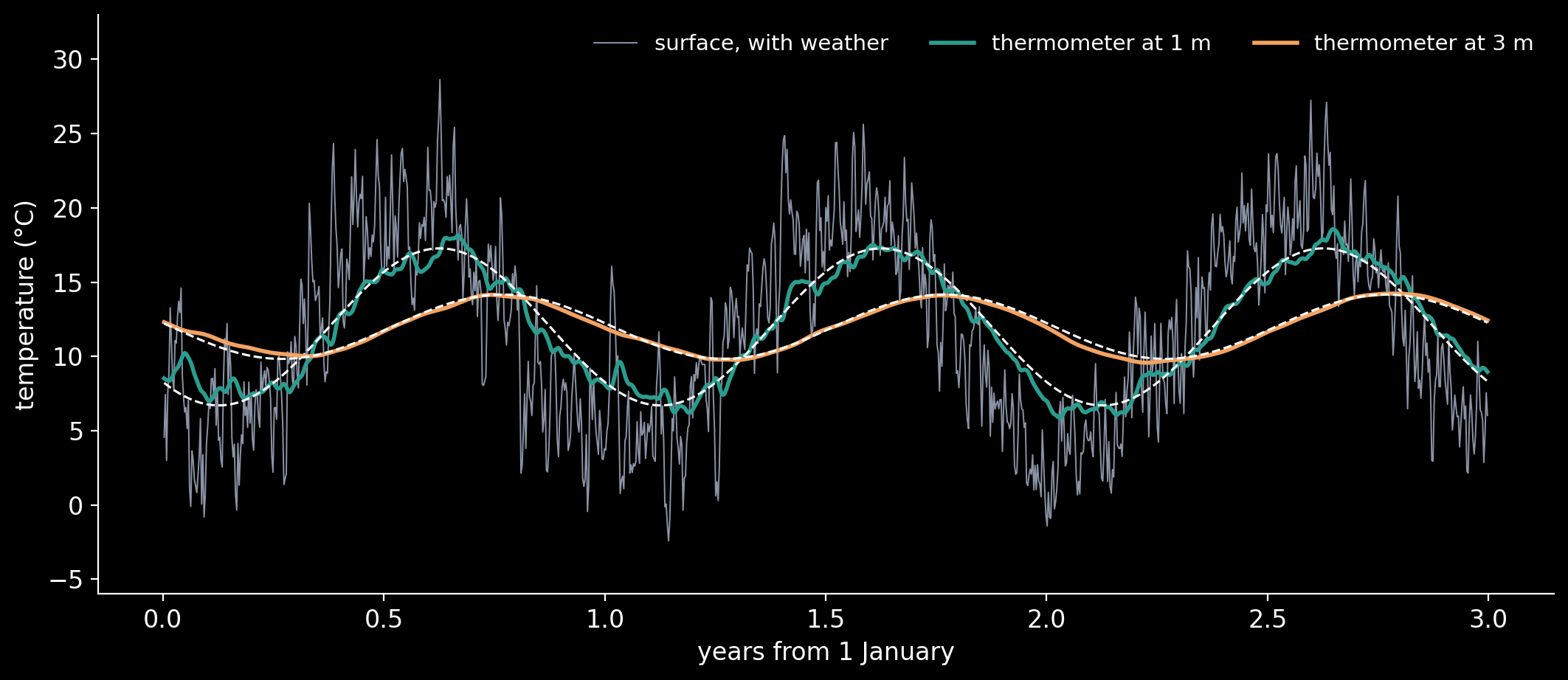
The test here is harder than the formula. The surface now has weather: day-to-day swings with a spread of 3 °C that persist from one day to the next (a correlation of 0.7). The grid carries the yearly wave and the weather down together, with the bottom held at the yearly mean, and two thermometers at 1 m and 3 m are read once a day for ten years. Fitting the yearly wave to each record gives its swing and its timing, and from them two estimates of $\kappa$, which should agree with each other and with the true value.
Kelvin’s Two Thermometers
def buried_records(seed, years, depths, spread=3.0, persist=0.7):
    rng = np.random.default_rng(seed)
    weather = np.zeros(int(round(years * YEAR)))
    for k in range(1, weather.size):
        shock = spread * np.sqrt(1 - persist**2) * rng.standard_normal()
        weather[k] = persist * weather[k - 1] + shock
    top = lambda t: exact(0.0, t) + weather[int(round(t)) - 1]
    z, _, _, kept = crank_nicolson(L, 600, 1.0, 0.0, weather.size,
                                   lambda z: exact(z, 0.0), top, lambda t: Tbar,
                                   keep=True)
    t = np.arange(1, weather.size + 1) * 1.0
    cols = [int(round(depth / (z[1] - z[0]))) for depth in depths]
    return t, kept[:, 0], kept[:, cols]

def yearly_wave(t, record):
    X = np.column_stack([np.ones_like(t), np.cos(omega * t), np.sin(omega * t)])
    c0, c1, c2 = np.linalg.lstsq(X, record, rcond=None)[0]
    return np.hypot(c1, c2), np.arctan2(c2, c1)          # swing, timing (radians)

def two_estimates(t, rec, gap=2.0):
    (A1, p1), (A2, p2) = yearly_wave(t, rec[:, 0]), yearly_wave(t, rec[:, 1])
    lag = (p2 - p1 + np.pi) % (2 * np.pi) - np.pi
    k_swing = omega * gap**2 / (2 * np.log(A1 / A2) ** 2)
    k_lag = omega * gap**2 / (2 * lag**2)
    return k_swing, k_lag

t_rec, surface, rec = buried_records(1860, 10, (1.0, 3.0))
k_swing, k_lag = two_estimates(t_rec, rec)
to_si = 1 / 86400
print(f"true kappa:            {kappa * to_si:.3e} m²/s")
for name, k in (("the swing ratio", k_swing), ("the time lag", k_lag)):
    off = 100 * (k / kappa - 1)
    print(f"{'from ' + name + ':':22s} {k * to_si:.3e} m²/s   ({off:+.2f}%)")

runs = []
for seed in range(20):
    t_s, _, rec_s = buried_records(seed, 10, (1.0, 3.0))
    runs.append(two_estimates(t_s, rec_s))
runs = np.array(runs) / kappa
print()
print("twenty weather histories, as a share of the true kappa:")
print(f"  swing ratio: {runs[:, 0].mean():.4f} ± {runs[:, 0].std():.4f}")
print(f"  time lag:    {runs[:, 1].mean():.4f} ± {runs[:, 1].std():.4f}")

# true kappa:            5.000e-07 m²/s
# from the swing ratio:  4.991e-07 m²/s   (-0.18%)
# from the time lag:     4.996e-07 m²/s   (-0.08%)
#
#
# twenty weather histories, as a share of the true kappa:
#   swing ratio: 1.0011 ± 0.0054
#   time lag:    1.0014 ± 0.0056
What the Ground Keeps
In damp soil the yearly wave keeps 64% of its swing with every metre and runs 26 days later: ±8 °C at the surface, ±2.10 °C at 3 m, and ±0.35 °C at 7 m, where the warmest day falls on 22 January and the coldest on 24 July. A cellar three metres down stays within a few tenths of a degree of the yearly mean at both ends of the year: 11.82 °C on 15 January, when the surface is at 4.08 °C, and 12.13 °C on 15 July, when the surface is at 19.88 °C. That is why it feels warm in winter and cool in summer, though its own seasons run about two and a half months late.
The grid solution matches Fourier’s formula to 1.22 × 10⁻⁴ °C with 5 cm layers and one-day steps, and the error falls by a factor of four each time both are halved: an observed order of 2.006, as a second-order scheme should give. The daily wave dies 19.11 times nearer the surface than the yearly one, which is Fourier’s nineteen. And two thermometers at 1 m and 3 m, read daily through ten years of weather, give the soil’s diffusivity back within 0.2%, both from how much the wave shrinks and from how late it arrives; over twenty different weather histories, the two estimates scatter by about half a percent around the true value.
Sources
- J. Fourier, Théorie analytique de la chaleur, Firmin Didot, Paris, 1822.
- J. Fourier, “Mémoire sur les températures du globe terrestre et des espaces planétaires”, Mémoires de l’Académie Royale des Sciences de l’Institut de France 7 (1827) 569–604; first printed in Annales de Chimie et de Physique 27 (1824).
- J. D. Forbes, “Account of some experiments on the temperature of the earth at different depths, and in different soils, near Edinburgh”, Transactions of the Royal Society of Edinburgh 16 (1846) 189–236.
- W. Thomson, “On the reduction of observations of underground temperature; with application to Professor Forbes’ Edinburgh observations, and the continued Calton Hill series”, Transactions of the Royal Society of Edinburgh 22 (1861) 405–427.
- J. Crank and P. Nicolson, “A practical method for numerical evaluation of solutions of partial differential equations of the heat-conduction type”, Proceedings of the Cambridge Philosophical Society 43 (1947) 50–67.
- H. S. Carslaw and J. C. Jaeger, Conduction of Heat in Solids, 2nd edition, Clarendon Press, Oxford, 1959.
Interested in applying these ideas to your work? Get in touch.