The Noise That Looks Like Correlation

By Dr. T. Zamrik  ·  October 1, 2026

Estimate the correlation matrix of 200 assets from 500 days of returns and it will show correlations even when there are none. Between assets that are truly independent, the sample correlations scatter around zero, and the largest of the 19,900 pairs looks like a real relationship. The eigenvalues of the matrix spread across a wide band, and random matrix theory says exactly how wide: Marchenko and Pastur derived the band in 1967. Everything inside it is indistinguishable from noise.

This notebook measures the band on pure noise, plants a market with sectors to see which eigenvalues rise above it, cleans the matrix by keeping only those, and then shows why it matters: a minimum-variance portfolio built on the raw matrix promises a risk it does not deliver, by an amount the theory predicts in advance.

Pure Noise

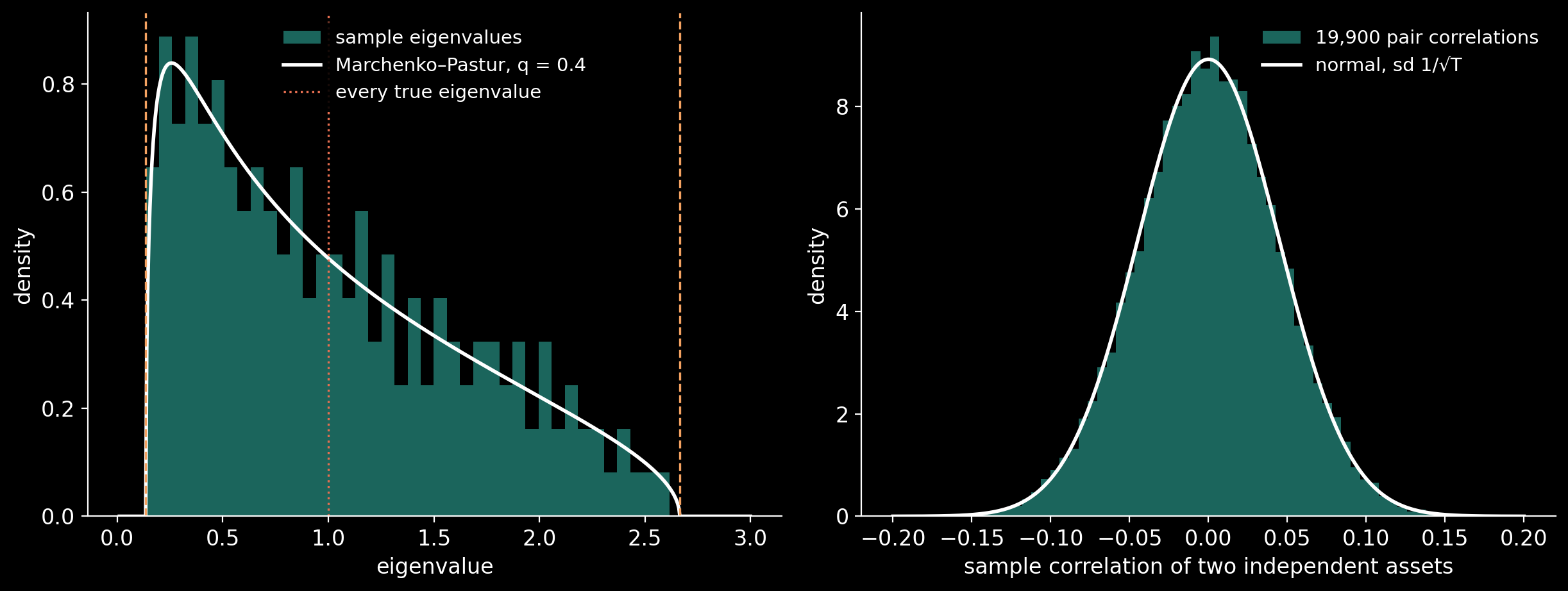
Two hundred assets, five hundred days, every return independent with unit variance. The ratio $q = N/T = 0.4$ sets the band in which the eigenvalues of the sample correlation matrix must fall, and the density inside it:

The true correlation matrix here is the identity: every true eigenvalue is exactly 1.

import numpy as np

N, T = 200, 500                       # assets, days
q = N / T
rng = np.random.default_rng(1967)     # the year of Marchenko and Pastur
X = rng.standard_normal((T, N))       # independent returns, unit variance
C = np.corrcoef(X, rowvar=False)      # the sample correlation matrix
lam = np.linalg.eigvalsh(C)
lo, hi = (1 - np.sqrt(q)) ** 2, (1 + np.sqrt(q)) ** 2
outside = np.sum((lam < lo) | (lam > hi))

print(f"q = N/T = {q}")
print(f"Marchenko-Pastur band: {lo:.4f} to {hi:.4f}")
print(f"sample eigenvalues:    {lam.min():.4f} to {lam.max():.4f}")
print(f"eigenvalues outside the band: {outside} of {N}")

# q = N/T = 0.4
# Marchenko-Pastur band: 0.1351 to 2.6649
# sample eigenvalues:    0.1362 to 2.6158
# eigenvalues outside the band: 0 of 200

Every true eigenvalue is 1, yet the sample ones run from about a seventh of that to more than two and a half times it. The same noise shows up pair by pair: a sample correlation between two independent series has a standard deviation of about $1/\sqrt{T}$, and with 19,900 pairs some of them are bound to look large.

iu = np.triu_indices(N, k=1)
r = C[iu]                             # every pair, once
print(f"pairs: {r.size}")
print(f"spread of the pair correlations: {r.std():.4f}")
print(f"theory, 1/sqrt(T):               {1 / np.sqrt(T):.4f}")
print(f"the largest |correlation|: {np.abs(r).max():.4f}")
print(f"pairs beyond 0.1 either way: {np.sum(np.abs(r) > 0.1)}")

# pairs: 19900
# spread of the pair correlations: 0.0447
# theory, 1/sqrt(T):               0.0447
# the largest |correlation|: 0.1853
# pairs beyond 0.1 either way: 513

A Market With Sectors

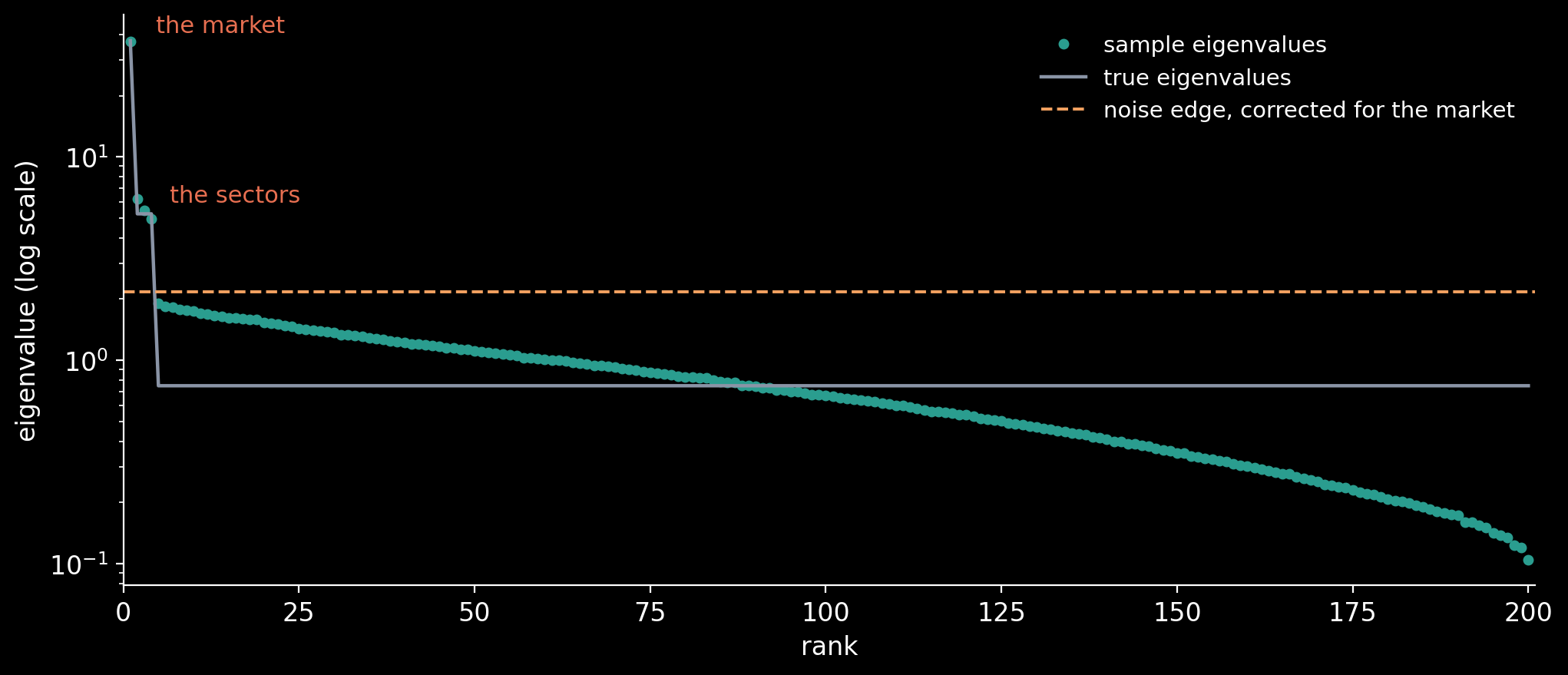
Now plant structure. Every asset loads 0.4 on one market factor, and each belongs to one of four sectors that adds a loading of 0.3 on its own factor; the rest is independent noise, so every asset still has unit variance. The true correlation matrix has exactly four eigenvalues above the rest: one for the market and three that tell the sectors apart. The question is whether the sample matrix shows four.

The edge of the noise band must first be corrected for the market, which carries a share of the total variance (Laloux and co-authors, 1999): the variance left for the noise is $\sigma^2 = 1 – \lambda_{\max}/N$, and the edge becomes $\sigma^2 (1 + \sqrt{q})^2$.

beta, gamma, K = 0.4, 0.3, 4          # market loading, sector loading, sectors
sector = np.arange(N) % K
idio = np.sqrt(1 - beta**2 - gamma**2)
m = rng.standard_normal((T, 1))
s = rng.standard_normal((T, K))
R = beta * m + gamma * s[:, sector] + idio * rng.standard_normal((T, N))

C_true = beta**2 + gamma**2 * (sector[:, None] == sector[None, :])
np.fill_diagonal(C_true, 1.0)
C_s = np.corrcoef(R, rowvar=False)
lam_t = np.linalg.eigvalsh(C_true)[::-1]
lam_s = np.linalg.eigvalsh(C_s)[::-1]
sigma2 = 1 - lam_s[0] / N             # the noise variance left after the market
edge = sigma2 * (1 + np.sqrt(q)) ** 2

show = lambda v: ", ".join(f"{x:.2f}" for x in v)
print(f"top true eigenvalues:   {show(lam_t[:6])}")
print(f"top sample eigenvalues: {show(lam_s[:6])}")
print(f"noise edge after the market: {edge:.4f}")
print(f"sample eigenvalues above it: {np.sum(lam_s > edge)}")

# top true eigenvalues:   37.25, 5.25, 5.25, 5.25, 0.75, 0.75
# top sample eigenvalues: 37.02, 6.24, 5.45, 4.97, 1.91, 1.83
# noise edge after the market: 2.1716
# sample eigenvalues above it: 4

Cleaning by Clipping

The simplest cure keeps what rises above the band and treats the rest as noise: the eigenvalues above the edge stay, every eigenvalue inside the band is replaced by their average so the trace stays the same, and the matrix is rebuilt and rescaled back to a correlation matrix (Laloux, Cizeau, Bouchaud and Potters, 1999). Because the truth is known here, the cleaning can be judged directly.

def clip(C, edge):
    w, V = np.linalg.eigh(C)
    noise = w <= edge
    w = w.copy()
    w[noise] = w[noise].mean()        # the bulk flattened, the trace kept
    Cc = (V * w) @ V.T
    d = np.sqrt(np.diag(Cc))
    return Cc / np.outer(d, d)        # back to a correlation matrix

C_c = clip(C_s, edge)
err = lambda A: np.linalg.norm(A - C_true) / np.linalg.norm(C_true)
print(f"distance to the truth, sample:  {err(C_s):.4f}")
print(f"distance to the truth, cleaned: {err(C_c):.4f}")

# distance to the truth, sample:  0.2075
# distance to the truth, cleaned: 0.1159

The Risk It Promises, and the Risk It Delivers

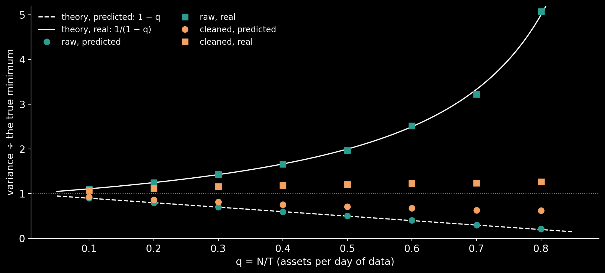
A minimum-variance portfolio weights the assets by $w \propto C^{-1}\mathbf{1}$, and the inverse amplifies the smallest eigenvalues, which are the noisiest. Its predicted variance is computed with the matrix it was built from; its real variance with the truth. For Gaussian returns the theory is exact in the limit: built on the raw sample covariance, the predicted variance is $(1-q)$ times the true minimum and the real one is $1/(1-q)$ times it (Pafka and Kondor, 2003). The portfolio believes it is safer than the best possible portfolio, and is in fact riskier.

Two hundred fresh samples are drawn from the planted market. Each builds a raw portfolio and a cleaned one, and each is scored both ways.

Lc = np.linalg.cholesky(C_true)
one = np.ones(N)
best = 1 / (one @ np.linalg.solve(C_true, one))   # the true minimum

def minvar(S):
    w = np.linalg.solve(S, one)
    return w / w.sum()

score = {"raw": [], "cleaned": []}
for _ in range(200):
    Z = rng.standard_normal((T, N)) @ Lc.T   # a fresh sample from the truth
    S = Z.T @ Z / T                          # its covariance (mean known: 0)
    d = np.sqrt(np.diag(S))
    Cz = S / np.outer(d, d)
    e = (1 - np.linalg.eigvalsh(Cz)[-1] / N) * (1 + np.sqrt(q)) ** 2
    S_c = clip(Cz, e) * np.outer(d, d)       # cleaned; sample vols kept
    for name, M in (("raw", S), ("cleaned", S_c)):
        w = minvar(M)
        score[name].append((w @ M @ w / best, w @ C_true @ w / best))

for name, v in score.items():
    p, r = np.mean(v, axis=0)
    print(f"{name:8s} predicted {p:.3f} x the minimum, real {r:.3f} x")
print(f"theory   predicted {1 - q:.3f} x the minimum, real {1 / (1 - q):.3f} x")

# raw      predicted 0.604 x the minimum, real 1.656 x
# cleaned  predicted 0.765 x the minimum, real 1.183 x
# theory   predicted 0.600 x the minimum, real 1.667 x

What the Noise Costs

With 200 assets and 500 days, all but four of the 200 eigenvalues of the planted market’s sample matrix sit in the band that pure noise would fill. A portfolio built on the raw matrix promises a variance 40% below the true minimum and delivers one 66% above it: 0.604 and 1.656 times the minimum, against 0.600 and 1.667 from the theory, written down before a single number is drawn. Clipping the band costs a few lines of code and brings the real variance down to 18% above the minimum. It does not create information, though: it only stops the optimiser from trading on noise.

Sources

1. V. A. Marčenko and L. A. Pastur, “Distribution of eigenvalues for some sets of random matrices”, Mathematics of the USSR-Sbornik 1 (1967) 457–483.
2. L. Laloux, P. Cizeau, J.-P. Bouchaud and M. Potters, “Noise dressing of financial correlation matrices”, Physical Review Letters 83 (1999) 1467–1470.
3. V. Plerou, P. Gopikrishnan, B. Rosenow, L. A. N. Amaral and H. E. Stanley, “Universal and nonuniversal properties of cross correlations in financial time series”, Physical Review Letters 83 (1999) 1471–1474.
4. S. Pafka and I. Kondor, “Noisy covariance matrices and portfolio optimization II”, Physica A 319 (2003) 487–494.
5. J. Bun, J.-P. Bouchaud and M. Potters, “Cleaning large correlation matrices: tools from random matrix theory”, Physics Reports 666 (2017) 1–109.

Working on a pricing model or risk system? Let’s talk.