
In February 1997 the National Weather Service gave Grand Forks, North Dakota, an outlook crest of 49 feet for the Red River of the North. The city built its dikes to about 52 feet. The river crested at 54.35 feet, and more than 50,000 people were evacuated.
This notebook recomputes what that 49 feet implied, from one table: the Weather Service’s own record of its spring outlooks. The arithmetic is Jensen’s inequality, and its verdict fits in a line: the damage of the average is not the average damage. The story of the flood is told in the blog post The Average That Drowned a City.
The Forecaster’s Record
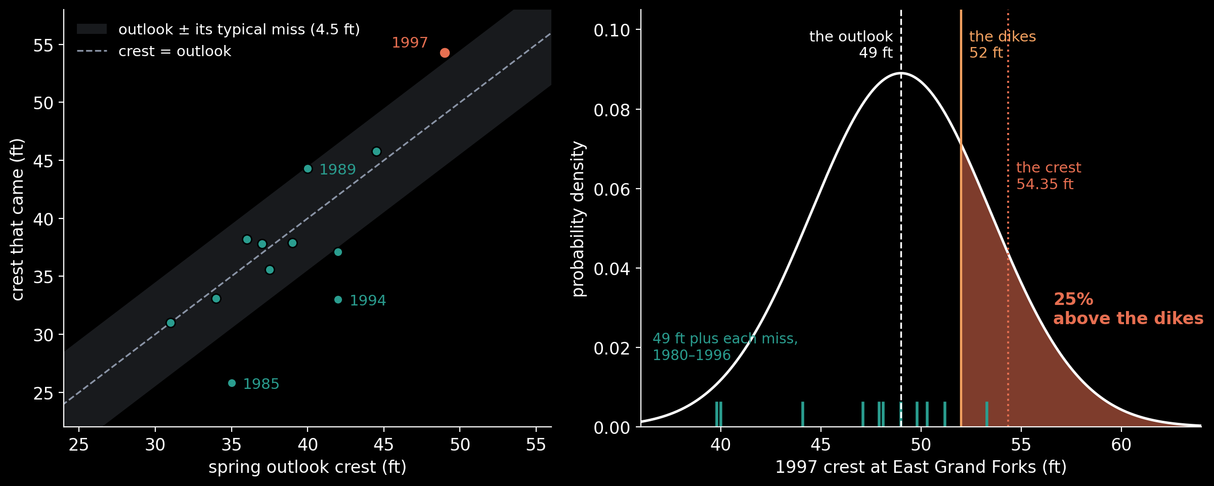
Table 3 of the Weather Service’s 1998 service assessment lists, for East Grand Forks, every spring outlook from 1980 to 1997 that assumed normal future precipitation, and the crest that followed. The Weather Service says such outlooks sit at about the median: a 50% chance of being equalled or exceeded.
The NWS Record, 1980–1997
import numpy as np
from math import erf, exp, pi, sqrt

# (outlook crest, crest that came) in feet, East Grand Forks,
# from the NWS 1998 service assessment, Table 3
record = {1980: (31.0, 31.0), 1982: (42.0, 37.1), 1984: (36.0, 38.2),
          1985: (35.0, 25.8), 1986: (39.0, 37.9), 1987: (34.0, 33.1),
          1989: (40.0, 44.3), 1993: (37.5, 35.6), 1994: (42.0, 33.0),
          1995: (37.0, 37.8), 1996: (44.5, 45.8), 1997: (49.0, 54.3)}
# the 1997 outlook, the dikes, and the crest usually quoted
forecast, dikes, crest = 49.0, 52.0, 54.35

print("year  outlook  crest   miss")
for year, (outlook, came) in record.items():
    print(f"{year}  {outlook:7.1f}  {came:5.1f}  {came - outlook:+5.1f}")

# year  outlook  crest   miss
# 1980     31.0   31.0   +0.0
# 1982     42.0   37.1   -4.9
# 1984     36.0   38.2   +2.2
# 1985     35.0   25.8   -9.2
# 1986     39.0   37.9   -1.1
# 1987     34.0   33.1   -0.9
# 1989     40.0   44.3   +4.3
# 1993     37.5   35.6   -1.9
# 1994     42.0   33.0   -9.0
# 1995     37.0   37.8   +0.8
# 1996     44.5   45.8   +1.3
# 1997     49.0   54.3   +5.3
Table 3 lists the 1997 crest as 54.3 feet; the crest usually quoted is 54.35. Only the eleven years before 1997 were known when the outlook was issued, so they alone set the typical miss: its root mean square.
Known in Spring 1997
before = {y: came - outlook for y, (outlook, came) in record.items() if y < 1997}
miss = np.array(list(before.values()))
s = sqrt((miss ** 2).mean())                  # the typical miss
met_all = sum(came >= outlook for outlook, came in record.values())

print(f"outlooks before 1997: {len(miss)}, met or beaten in {(miss >= 0).sum()}")
print(f"all twelve, 1997 included: met or beaten in {met_all}")
print(f"misses from {miss.min():+.1f} ft to {miss.max():+.1f} ft")
print(f"mean miss {miss.mean():+.2f} ft, typical miss {s:.2f} ft")

# outlooks before 1997: 11, met or beaten in 5
# all twelve, 1997 included: met or beaten in 6
# misses from -9.2 ft to +4.3 ft
# mean miss -1.67 ft, typical miss 4.48 ft
Jensen’s Inequality at 52 Feet
Write $H$ for the 1997 crest, still uncertain in February, and measure the damage as the depth of water over the dikes. The damage is convex, flat below the dikes and rising beyond them, so Jensen’s inequality applies:
The city’s arithmetic was the right-hand side: the forecast put into the damage. What it needed was the left-hand side. Take the outlook as the median and the typical miss as the spread, $H \sim N(\mu, \sigma^2)$ with $\mu = 49$ feet and dikes at $L = 52$ feet, and the expected depth over the dikes has a closed form:
The Damage of the Average, and the Average Damage
Phi = lambda z: 0.5 * (1 + erf(z / sqrt(2)))
phi = lambda z: exp(-z * z / 2) / sqrt(2 * pi)

def damage(h):                      # feet of water over the dikes: convex
    return max(0.0, h - dikes)

def expected_damage(sigma):         # E[damage(H)] for H ~ N(forecast, sigma^2)
    z = (dikes - forecast) / sigma
    return sigma * phi(z) - (dikes - forecast) * (1 - Phi(z))

def p_over(sigma, height=dikes):    # the chance the crest tops dikes of this height
    return 1 - Phi((height - forecast) / sigma)

print(f"D(E[H]), the damage at the forecast: {damage(forecast):.2f} ft")
print(f"E[D(H)], the expected damage:        {expected_damage(s):.3f} ft")
print(f"chance the crest tops the dikes:     {p_over(s):.1%}")

# D(E[H]), the damage at the forecast: 0.00 ft
# E[D(H)], the expected damage:        0.674 ft
# chance the crest tops the dikes:     25.2%
The normal shape is an assumption. Drop it, and replay the eleven real misses on top of 49 feet exactly as they happened:
The Eleven Misses, Replayed
replayed = forecast + miss
over = [y for y, e in before.items() if forecast + e > dikes]
n, k = len(over), len(miss)
print(f"replayed crests above the dikes: {n} of {k} ({n / k:.1%}),"
      f" from {over[0]}")
depth = np.maximum(replayed - dikes, 0).mean()
print(f"expected depth over the dikes: {depth:.3f} ft")

# replayed crests above the dikes: 1 of 11 (9.1%), from 1989
# expected depth over the dikes: 0.118 ft
One in four, or one in eleven: the replay is lower because the outlooks had more often erred high than low. Neither is zero. A million crests drawn from the normal, seeded, check the closed form:
A Million Crests
rng = np.random.default_rng(19970422)
H = forecast + s * rng.standard_normal(1_000_000)
p_mc, depth_mc = (H > dikes).mean(), np.maximum(H - dikes, 0).mean()
print(f"Monte Carlo: tops the dikes {p_mc:.4f}, expected depth {depth_mc:.4f} ft")
p_cf, depth_cf = p_over(s), expected_damage(s)
print(f"closed form: tops the dikes {p_cf:.4f}, expected depth {depth_cf:.4f} ft")

# Monte Carlo: tops the dikes 0.2514, expected depth 0.6741 ft
# closed form: tops the dikes 0.2516, expected depth 0.6742 ft
The Gap Is Curvature Times Variance
Expand any smooth $f$ around the mean, and Jensen’s gap is the curvature times the variance:
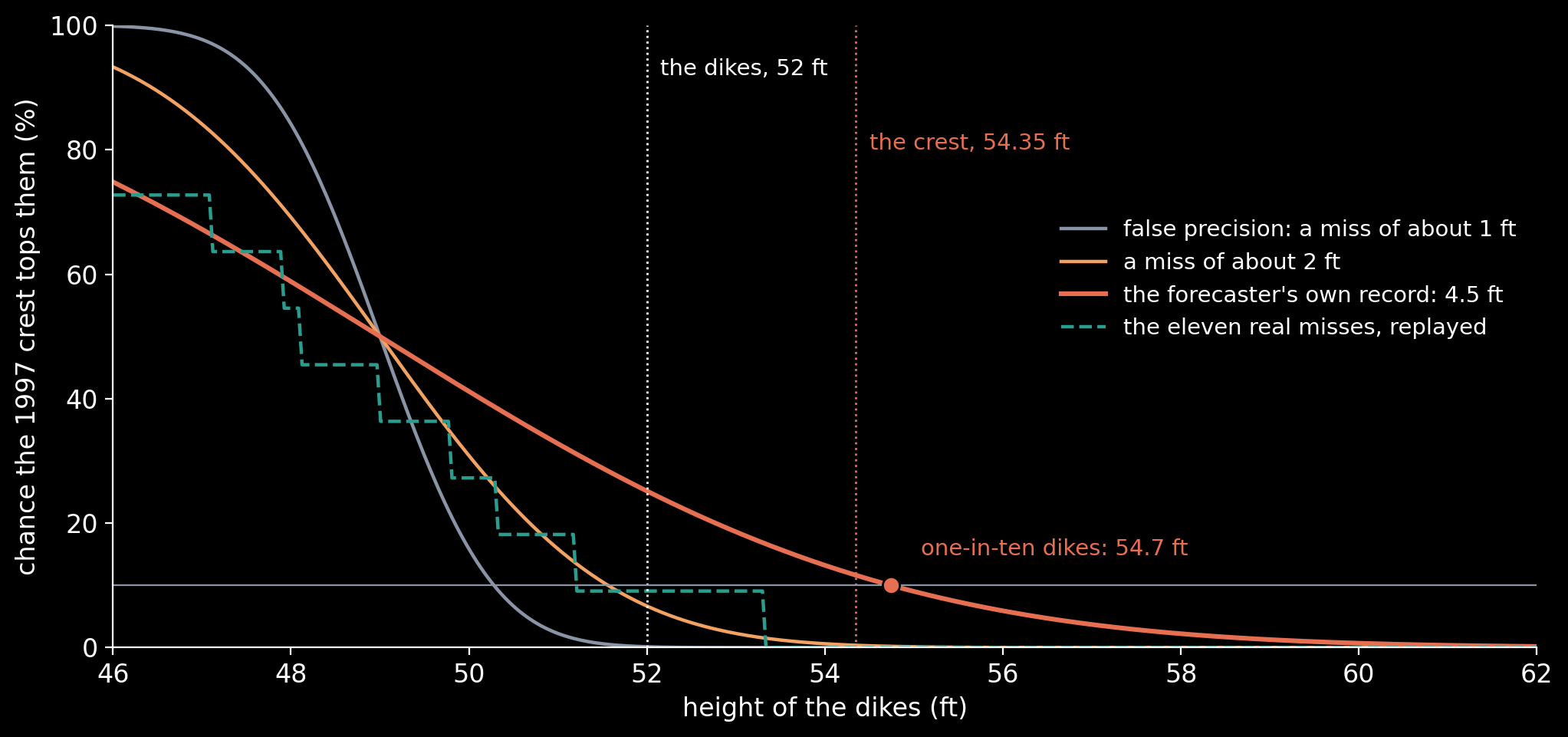
The curvature belongs to the city: where its dikes stand. The variance belongs to the forecast. A single number has a variance of zero, and so a gap of zero. Same median, same dikes, and only the typical miss changing:
The Variance Is the Whole Gap
print("typical miss   tops the dikes   expected depth")
for sigma in (0.5, 1.0, 2.0, 3.0, s):
    p, depth = p_over(sigma), expected_damage(sigma)
    print(f"{sigma:8.2f} ft   {p:14.2%}   {depth:11.4f} ft")

# typical miss   tops the dikes   expected depth
#     0.50 ft            0.00%        0.0000 ft
#     1.00 ft            0.13%        0.0004 ft
#     2.00 ft            6.68%        0.0586 ft
#     3.00 ft           15.87%        0.2499 ft
#     4.48 ft           25.16%        0.6742 ft
The Dikes the Record Asked For
Choose the risk first, and the record gives the height:
Dikes for a Chosen Risk
# the normal's 90% and 95% points
for odds, z in (("one in ten", 1.2815515655446004),
                ("one in twenty", 1.6448536269514722)):
    print(f"dikes for a {odds} chance of being topped: {forecast + z * s:.1f} ft")
above = (crest - forecast) / s
print(f"the crest, {crest} ft, was {above:.2f} typical misses above the outlook")

# dikes for a one in ten chance of being topped: 54.7 ft
# dikes for a one in twenty chance of being topped: 56.4 ft
# the crest, 54.35 ft, was 1.19 typical misses above the outlook
The 49 feet was not a bad forecast. It was a median, and it said so. Put a median into a convex loss and the answer is zero; average the loss over the forecaster’s own record and it is a one-in-four chance of water over the dikes. The Weather Service now gives its Red River outlooks as chances of exceeding each level, not as one number to build to.
Sources
- National Weather Service, Red River of the North 1997 Floods: Service Assessment and Hydraulic Analysis, U.S. Department of Commerce, National Oceanic and Atmospheric Administration (August 1998), Table 3.
- J. L. W. V. Jensen, “Sur les fonctions convexes et les inégalités entre les valeurs moyennes”, Acta Mathematica 30 (1906) 175–193.
Interested in applying these ideas to your work? Get in touch.