
In the summer of 1991 the first issue of The Journal of Fixed Income carried an eight-page paper by Robert Litterman, then a vice president in fixed income research at Goldman Sachs in New York, and José Scheinkman, the Alvin Baum Professor of Economics at the University of Chicago. Its title was plain, “Common Factors Affecting Bond Returns”, and so was its claim. Treasury bonds of every maturity, from a few months to thirty years, each with its own price every day, move as if only three things were pushing them: the whole curve shifting up or down, the curve getting steeper or flatter, and its middle bending against its two ends. They called the three level, steepness and curvature.
The paper sits behind the journal’s paywall and was not read for this notebook, so its numbers appear here in the words of those who reported them. Robert Bliss of the Federal Reserve Bank of Atlanta wrote in 1997 that “Of Litterman and Scheinkman’s three factors, the first one accounted for an average of 89.5 percent of the observed variation in yield changes across maturities”, and that their data were “weekly returns for thirteen Treasury bonds of maturities ranging from six months to nearly thirty years over the period from February 1984 through August 1988.” In a 2003 Economic Letter of the Federal Reserve Bank of San Francisco, Tao Wu wrote that “empirical studies reveal that more than 99% of the movement of various Treasury bond yields are captured by three factors”, citing the paper.
It mattered to anyone who holds bonds against other bonds. The usual hedge matched duration, which protects a position against a parallel shift of the curve, close to what the first factor does, and leaves the other two open. In Bliss’s account, “Litterman and Scheinkman show that hedging based on three factors will improve hedge performance relative to Macaulay duration–based hedging by 28 percent on average and in some cases much more.”
Thirty-five years and three regimes later (the 1990s; seven years in which the Federal Reserve held its policy rate at zero; then eleven increases that took it from zero to 5¼–5½ percent in sixteen months) this notebook measures it again on the Treasury’s own daily curve, January 1990 to October 2026. Is it still three numbers? Did the years at zero break the pattern? And what does a trader who hedges only the level still carry?
The Treasury’s Own Curve
Every business day the U.S. Treasury publishes its par yield curve: for each fixed maturity, the yield of a security priced at its face value, “the par yield for a new theoretical 20-year bond”, in Treasury’s example. No security has exactly those maturities on most days, so the curve is fitted to indicative bid-side price quotations for the most recently auctioned bills, notes and bonds, taken at about 3:30 PM each trading day: in Treasury’s words “a par yield curve derived using a monotone convex method”, the method in use since 6 December 2021, after a quasi-cubic Hermite spline.
The file holds every published value from 2 January 1990 to 14 October 2026, in percent, exactly as published; a maturity not published on a day is left empty. Some maturities came later: the 20-year on 1 October 1993, the 1-month on 31 July 2001, the 2-month on 16 October 2018, the 4-month on 19 October 2022 and the 1.5-month on 18 February 2025. The 30-year is missing from 19 February 2002 to 8 February 2006: Treasury’s series “was discontinued on February 18, 2002 and reintroduced on February 9, 2006.” Eight maturities run unbroken through the whole span, from three months to ten years, and they are the curve of this notebook. A daily change is taken only between two consecutive published days that carry all eight, in basis points (a hundredth of a percentage point).
The Treasury’s Own Curve
import numpy as np
import pandas as pd

df = pd.read_csv("data/treasury_par_yields.csv", index_col="date",
                 parse_dates=True)
CORE = ["3M", "6M", "1Y", "2Y", "3Y", "5Y", "7Y", "10Y"]
YRS = {"1M": 1/12, "1.5M": 1.5/12, "2M": 2/12, "3M": 0.25, "4M": 1/3,
       "6M": 0.5, "1Y": 1, "2Y": 2, "3Y": 3, "5Y": 5, "7Y": 7, "10Y": 10,
       "20Y": 20, "30Y": 30}           # each maturity in years

def changes(cols, start=None, end=None):
    # day-to-day changes in basis points, only between two consecutive
    # published days that both carry every maturity in cols
    d = df.dropna(how="all")[cols].diff() * 100
    return d.dropna().loc[start:end]

print(f"{len(df):,} days, {df.index[0]:%d %b %Y} to {df.index[-1]:%d %b %Y}")
print(f"{'maturity':>8}{'first day':>13}{'days':>7}{'empty since':>13}")
for c in df.columns:
    s = df[c]
    first = s.first_valid_index()
    print(f"{c:>8}{first.strftime('%d %b %Y'):>13}{s.notna().sum():>7,}"
          f"{s[first:].isna().sum():>13,}")
dy = changes(CORE)
print(f"\n{len(dy):,} daily changes of the eight from {dy.index[0]:%d %b %Y}")
print("one standard deviation of a day's change, basis points:")
print("  ".join(f"{c} {dy[c].std():.2f}" for c in CORE))

# 9,203 days, 02 Jan 1990 to 14 Oct 2026
# maturity    first day   days  empty since
#       1M  31 Jul 2001  6,303            1
#     1.5M  18 Feb 2025    415            0
#       2M  16 Oct 2018  1,998            0
#       3M  02 Jan 1990  9,199            4
#       4M  19 Oct 2022    996            0
#       6M  02 Jan 1990  9,202            1
#       1Y  02 Jan 1990  9,202            1
#       2Y  02 Jan 1990  9,202            1
#       3Y  02 Jan 1990  9,202            1
#       5Y  02 Jan 1990  9,202            1
#       7Y  02 Jan 1990  9,202            1
#      10Y  02 Jan 1990  9,202            1
#      20Y  01 Oct 1993  8,263            1
#      30Y  02 Jan 1990  8,208          995
#
# 9,195 daily changes of the eight from 03 Jan 1990
# one standard deviation of a day's change, basis points:
# 3M 4.59  6M 4.02  1Y 4.48  2Y 5.60  3Y 5.86  5Y 6.10  7Y 6.08  10Y 5.78
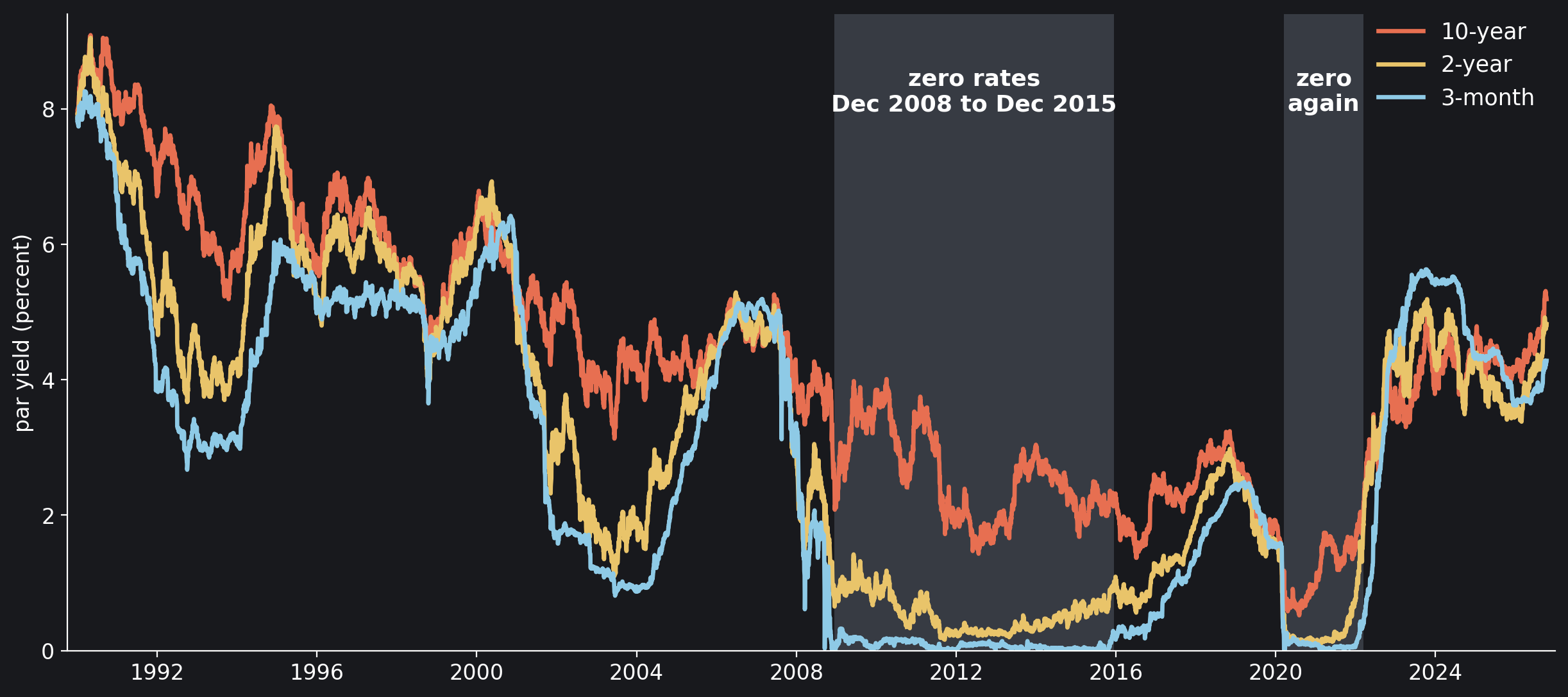
Of the 9,203 published days, one, 11 October 2010, carries no yields at all, and on three days of December 2008 the 3-month is empty; that leaves 9,195 daily changes of the eight. A typical day moves the 10-year yield by 5.78 basis points and the 3-month bill by 4.59, and the middle of the curve moves most: the 5-year by 6.10. Figure 1 shows the three that tell the story: the 3-month bill, which follows the Federal Reserve’s policy rate, the 2-year and the 10-year.
The Three Shapes
Stack the eight changes of day $t$ in one vector $\Delta y_t \in \mathbb{R}^8$. Over the $T$ days, their covariance matrix and its eigen-decomposition are
Each column of $V$ is a shape, a pattern of moves across the eight maturities; each eigenvalue $\lambda_k$ is the variance that shape carries, and its share of the total is $\lambda_k / \sum_j \lambda_j$. The scores
say how much of each shape day $t$ held. The covariance matrix is used rather than the correlation matrix because the eight changes are in one unit, basis points: a maturity that moves more should weigh more, and correlations would give each maturity the same say however much it moves. A shape and its negative are the same shape, so each is turned until its largest entry is positive.
The Three Shapes
NAMES = ["level", "steepness", "curvature"]

def shapes(d):
    # the shares of variance, largest first, and the shapes V (columns)
    lam, V = np.linalg.eigh(np.cov(np.asarray(d), rowvar=False))
    lam, V = lam[::-1], V[:, ::-1]
    top = np.abs(V).argmax(0)          # each shape's largest entry ...
    V = V * np.sign(V[top, range(V.shape[1])])   # ... made positive
    return lam / lam.sum(), V

share, V = shapes(dy)
for k in range(3):
    print(f"{NAMES[k]:<10} {share[k]:6.1%}")
print(f"{'all three':<10} {share[:3].sum():6.1%}   "
      f"the other five {share[3:].sum():.1%}")
print(f"\n{'':10}" + "".join(f"{c:>7}" for c in CORE))
for k in range(3):
    print(f"{NAMES[k]:<10}" + "".join(f"{x:>+7.2f}" for x in V[:, k]))

# level       79.4%
# steepness   12.7%
# curvature    4.1%
# all three   96.2%   the other five 3.8%
#
#                3M     6M     1Y     2Y     3Y     5Y     7Y    10Y
# level       +0.15  +0.20  +0.28  +0.39  +0.42  +0.44  +0.43  +0.39
# steepness   +0.68  +0.49  +0.33  +0.08  -0.03  -0.18  -0.26  -0.29
# curvature   +0.53  +0.01  -0.36  -0.48  -0.29  +0.06  +0.30  +0.43
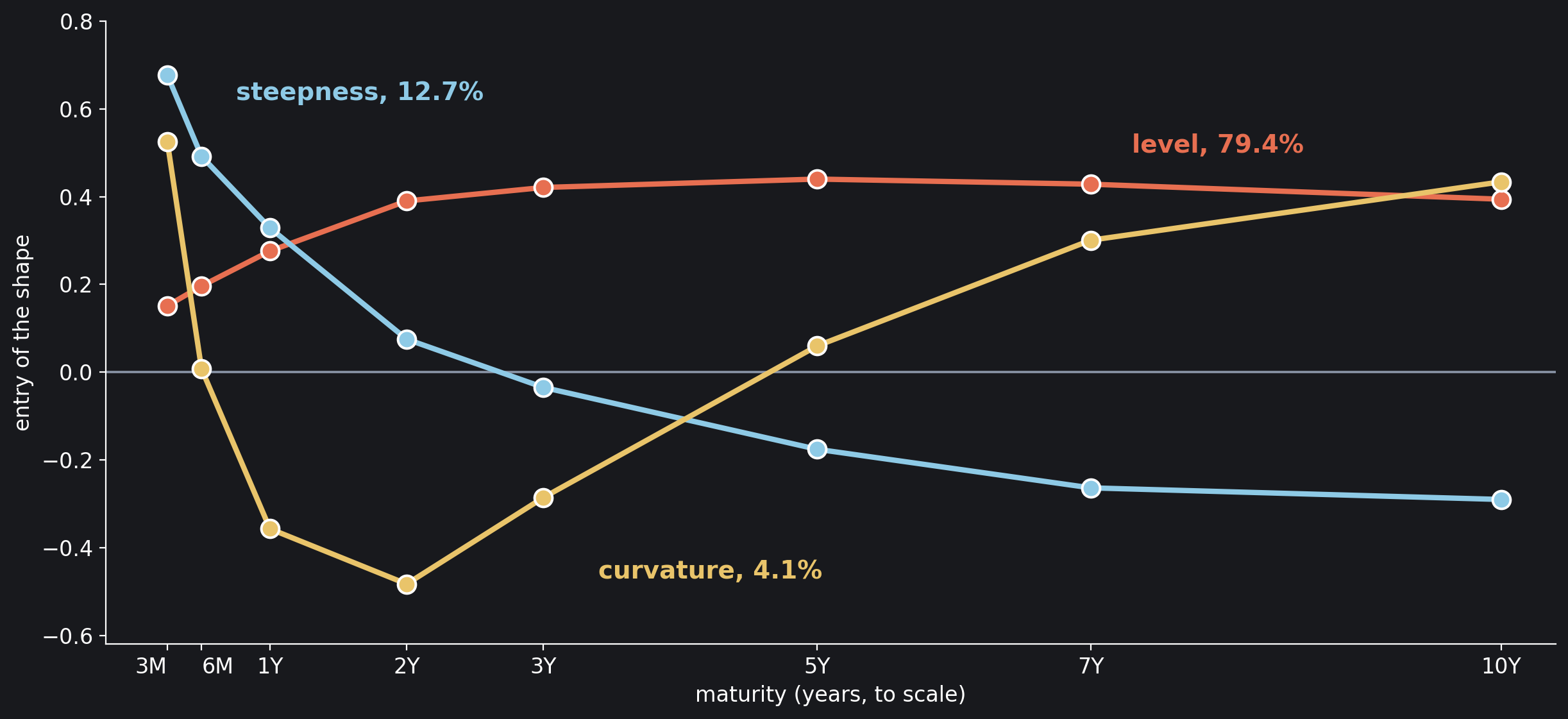
Three shapes carry 96.2% of the variance of the daily changes: level 79.4%, steepness 12.7%, curvature 4.1%; the other five shapes share the last 3.8%. The level is not a parallel shift. Every maturity moves the same way, but the 3-month moves 0.15 for every 0.44 of the 5-year, and the 10-year 0.39: in the level move the middle of the curve moves most. Steepness lifts the short end (+0.68 at three months) and lowers the long end (−0.29 at ten years), crossing zero between two and three years. Curvature lifts both ends, +0.53 and +0.43, against a dip of −0.48 at two years. Figure 2 draws the three.
Is It Still Three?
The same decomposition, era by era: the 1990s; 2000 to the eve of the zero-rate years; those years, from the Federal Open Market Committee’s statement of 16 December 2008, “The Federal Open Market Committee decided today to establish a target range for the federal funds rate of 0 to 1/4 percent”, to that of 16 December 2015, “the Committee decided to raise the target range for the federal funds rate to 1/4 to 1/2 percent”; the six years after; and from 2022, which holds the hiking cycle. The last two columns are each era’s level entries at three months and at ten years.
Era by Era
ERAS = {"1990-1999": ("1990", "1999"),
        "2000-2008": ("2000", "2008-12-15"),
        "zero rates": ("2008-12-16", "2015-12-16"),
        "2016-2021": ("2015-12-17", "2021"),
        "2022 on": ("2022", None)}
print(f"{'':11}{'days':>6}{'level':>8}{'steep':>8}{'curve':>8}{'three':>8}"
      f"{'3M':>7}{'10Y':>7}")
for era, (a, b) in ERAS.items():
    d = dy.loc[a:b]
    s, W = shapes(d)
    print(f"{era:11}{len(d):>6,}" + "".join(f"{x:>8.1%}" for x in s[:3])
          + f"{s[:3].sum():>8.1%}{W[0, 0]:>+7.2f}{W[-1, 0]:>+7.2f}")

#              days   level   steep   curve   three     3M    10Y
# 1990-1999   2,502   83.3%   10.4%    2.7%   96.4%  +0.19  +0.37
# 2000-2008   2,238   76.1%   17.1%    3.4%   96.6%  +0.22  +0.35
# zero rates  1,749   89.0%    5.9%    1.7%   96.6%  +0.01  +0.52
# 2016-2021   1,511   80.0%    9.8%    4.6%   94.4%  +0.08  +0.48
# 2022 on     1,195   85.0%    8.1%    3.7%   96.8%  +0.09  +0.36
In every era three shapes carry between 94.4% and 96.8%. The zero-rate years do not break the count; they move the weight. The level carries 89.0% there, more than in any other era, and steepness falls to 5.9%. The policy rate pinned the short end, and with the short end still, there was little left to steepen.
By calendar year the count stays close to three as well. Since the 1991 paper’s own data were weekly, the next cell also takes weekly changes, Friday to Friday, the whole period and each year. Its last line is the comparison as near as this file allows to the paper’s: weekly changes in the 1990s, the maturities from six months, and for each maturity the share of its own variance that the level explains, averaged over the maturities, the way Bliss describes their 89.5%.
Year by Year
def left(d, W, k):
    # share of each maturity's variance left after the first k shapes
    X = np.asarray(d)
    R = X - X @ W[:, :k] @ W[:, :k].T  # the residual
    return R.var(0) / X.var(0)

weekly = (df[CORE].dropna().resample("W-FRI").last().diff() * 100).dropna()
rows = []
for y in range(1990, dy.index[-1].year + 1):
    sd, _ = shapes(dy[dy.index.year == y])
    sw, _ = shapes(weekly[weekly.index.year == y])
    rows.append((y, sd[0], sd[:3].sum(), sw[:3].sum()))
by_year = pd.DataFrame(rows, columns=["year", "level", "three",
                                      "three_weekly"]).set_index("year")
for col, name in (("three", "daily"), ("three_weekly", "weekly")):
    t = by_year[col]
    n99 = (t >= 0.99).sum()
    print(f"{name}, three shapes by year: {t.min():.1%} ({t.idxmin()}) to "
          f"{t.max():.1%} ({t.idxmax()}), {n99} of {len(t)} at 99%")
for name, a, b in (("whole period", None, None), ("1990s", "1990", "1999")):
    s, _ = shapes(weekly.loc[a:b])
    print(f"weekly, {name}: level {s[0]:.1%}, three shapes {s[:3].sum():.1%}")
w90 = weekly.loc["1990":"1999", CORE[1:]]     # 6 months to 10 years
s, W = shapes(w90)
own1, own3 = 1 - left(w90, W, 1), 1 - left(w90, W, 3)
print("weekly 1990s, 6M to 10Y, share of each maturity's own variance:")
print(f"  level {own1.mean():.1%} on average; three shapes {own3.mean():.1%}, "
      f"from {own3.min():.1%} to {own3.max():.1%}")

# daily, three shapes by year: 92.0% (2017) to 98.4% (2007), 0 of 37 at 99%
# weekly, three shapes by year: 95.4% (2008) to 99.1% (2003), 1 of 37 at 99%
# weekly, whole period: level 81.0%, three shapes 97.4%
# weekly, 1990s: level 86.1%, three shapes 97.8%
# weekly 1990s, 6M to 10Y, share of each maturity's own variance:
#   level 88.3% on average; three shapes 98.6%, from 96.9% to 99.1%
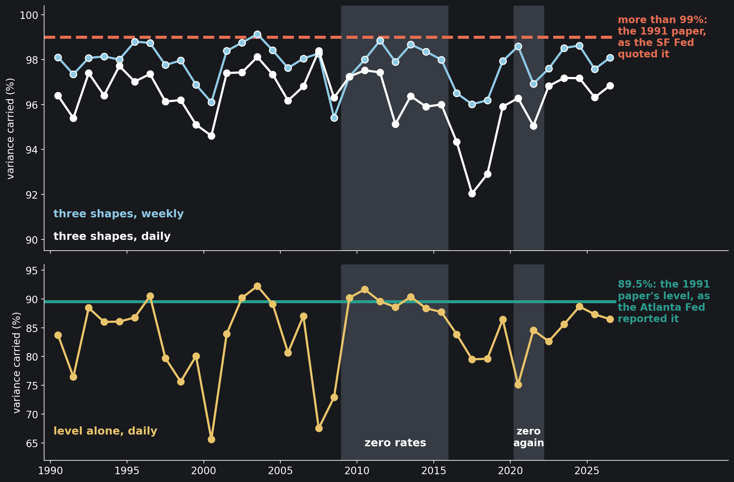
On daily changes, three shapes carry between 92.0% of a year’s variance (2017) and 98.4% (2007), and no calendar year of the 37 reaches 99%. Weekly changes are smoother: 97.4% over the whole period and 97.8% in the 1990s, and year by year from 95.4% (2008) to 99.1% (2003), the one year of 37 that reaches 99%. Bliss’s own study, monthly changes of zero-coupon yields since 1970, found the same steadiness: “Since 1978 the yield-change variation explained by three factors has remained between 95 and 98 percent.”
The comparison closest to the 1991 paper lands near it. Weekly, in the 1990s, from six months to ten years, the level explains on average 88.3% of each maturity’s own variance, against the 89.5% Bliss reports for Litterman and Scheinkman’s 1984–1988 sample; the three shapes explain 98.6% on average, between 96.9% and 99.1% maturity by maturity. Figure 3 sets the years against the two numbers quoted from the paper, each on its own measure.
When the Short End Could Not Move
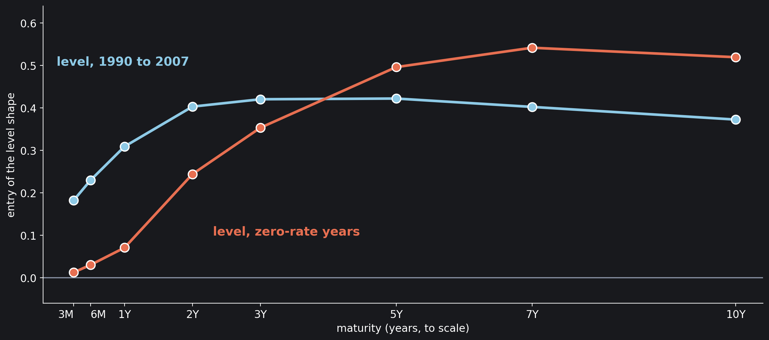
The count of shapes survived the zero-rate years; the first shape did not. Treasury floors its published curve at zero (“the derived par yield curve from these input prices for the Treasury nominal Constant Maturity Treasury series (CMTs) will be floored at zero”), and with the policy rate at 0 to ¼ percent the bills had almost nowhere to go. The level shape before 2008 and during those years, side by side:
When the Short End Could Not Move
V_before = shapes(dy.loc[:"2007"])[1][:, 0]
V_zero = shapes(dy.loc["2008-12-16":"2015-12-16"])[1][:, 0]
V_after = shapes(dy.loc["2022":])[1][:, 0]
print(f"{'level shape':17}" + "".join(f"{c:>6}" for c in CORE))
for name, v in (("1990-2007", V_before), ("zero rates", V_zero),
                ("2022 on", V_after)):
    print(f"{name:17}" + "".join(f"{x:>+6.2f}" for x in v))
print("\na day's change of the 3-month bill, one standard deviation:")
for era, (a, b) in ERAS.items():
    print(f"  {era:11} {dy.loc[a:b, '3M'].std():5.2f} basis points")

# level shape          3M    6M    1Y    2Y    3Y    5Y    7Y   10Y
# 1990-2007         +0.18 +0.23 +0.31 +0.40 +0.42 +0.42 +0.40 +0.37
# zero rates        +0.01 +0.03 +0.07 +0.24 +0.35 +0.50 +0.54 +0.52
# 2022 on           +0.09 +0.17 +0.31 +0.43 +0.44 +0.43 +0.41 +0.36
#
# a day's change of the 3-month bill, one standard deviation:
#   1990-1999    4.82 basis points
#   2000-2008    6.95 basis points
#   zero rates   1.22 basis points
#   2016-2021    2.32 basis points
#   2022 on      3.75 basis points
Before 2008 the level moved every maturity, from 0.18 at three months to 0.42 at three and five years. In the zero-rate years the 3-month entry fell to +0.01 and the 6-month to +0.03, while the 7-year and 10-year rose to 0.54 and 0.52: “level” had become a move of the long end alone. A day’s change of the 3-month bill shrank from 4.82 basis points in the 1990s, and 6.95 in 2000–2008, to 1.22. The shape came back with the rate: from 2022 the level runs from 0.09 at three months to 0.44 at three years, close to its old form with a quieter short end. Figure 4 draws the two shapes.
Hedge the Level Only
A position in one maturity, hedged against the first $k$ shapes with offsetting positions elsewhere on the curve, keeps only the part of its move that those shapes do not explain. For the whole curve that part is the residual
and the share of maturity $j$’s daily variance left is $\mathrm{var}(e_{t,j}) / \mathrm{var}(\Delta y_{t,j})$. With $k = 1$ the hedge covers the level alone; with $k = 3$, all three shapes.
Hedge the Level Only
left1, left3 = left(dy, V, 1), left(dy, V, 3)
print(f"{'maturity':>8}{'daily s.d. (bp)':>17}{'left, level':>14}"
      f"{'left, three':>14}")
for j, c in enumerate(CORE):
    print(f"{c:>8}{dy[c].std():>17.2f}{left1[j]:>14.1%}{left3[j]:>14.1%}")

# maturity  daily s.d. (bp)   left, level   left, three
#       3M             4.59         80.1%          4.2%
#       6M             4.02         56.4%         12.5%
#       1Y             4.48         30.3%          8.6%
#       2Y             5.60         11.0%          3.5%
#       3Y             5.86          5.6%          3.3%
#       5Y             6.10          4.6%          2.0%
#       7Y             6.08          9.1%          1.3%
#      10Y             5.78         14.9%          2.3%
Hedged against the level alone, a 5-year position keeps 4.6% of its daily variance, a 2-year 11.0% and a 10-year 14.9%; the 3-month bill keeps 80.1%, because the level hardly touches it. Hedged against all three shapes, the 5-year keeps 2.0%, the 2-year 3.5% and the 10-year 2.3%. In standard deviations, a 10-year position hedged on the level alone still moves by $5.78\sqrt{0.149} = 2.2$ basis points a day.
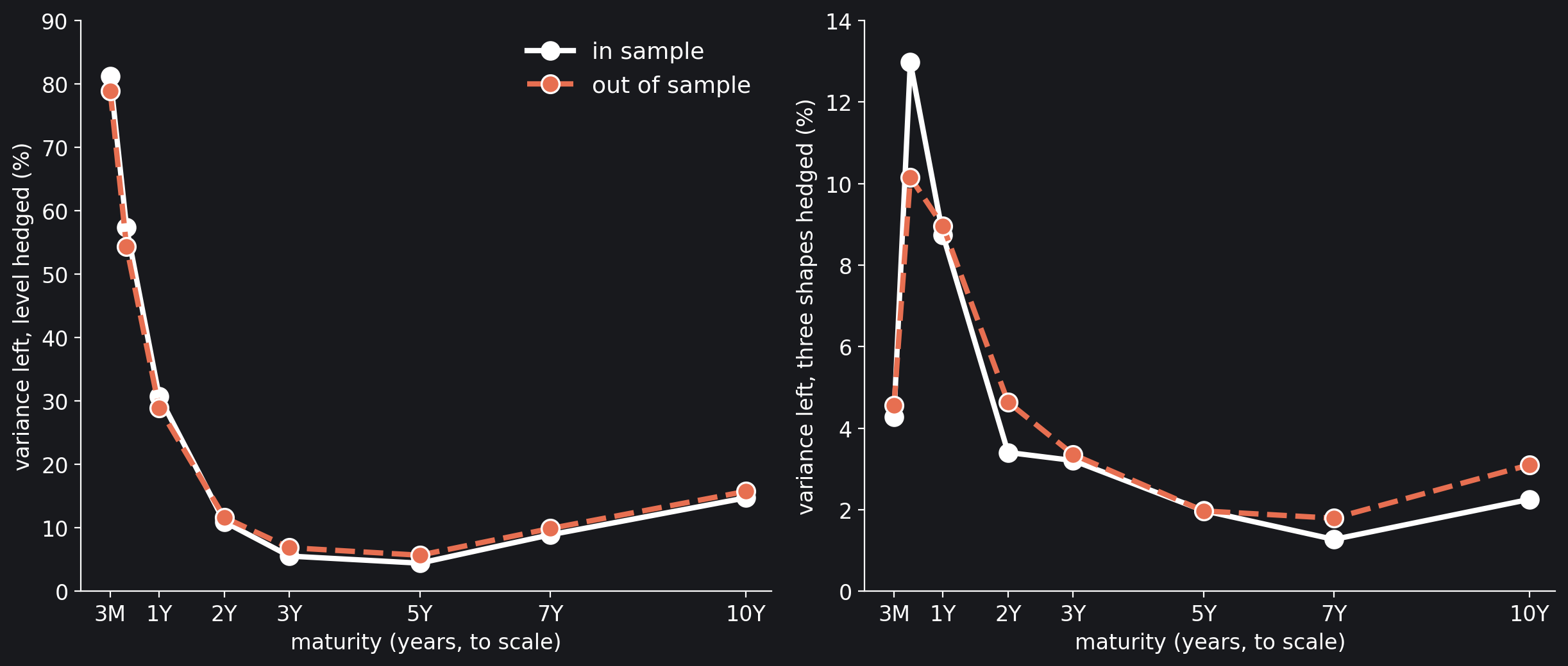
These are in-sample numbers: the shapes were estimated on the same days they are tested on, which flatters them. The honest version estimates the shapes on the previous 500 trading days, about two years, applies them to the next 250 without looking, and rolls forward through the whole sample.
Out of Sample
EST, APPLY = 500, 250                  # days to estimate, days to apply
X = dy.to_numpy()
res = {1: [], 3: []}
for s in range(EST, len(X), APPLY):
    _, W = shapes(X[s - EST:s])        # shapes from the past only
    B = X[s:s + APPLY]
    for k in res:
        res[k].append(B - B @ W[:, :k] @ W[:, :k].T)
B = X[EST:]                            # every day tested out of sample
oos = {k: np.vstack(r).var(0) / B.var(0) for k, r in res.items()}
ins = {k: left(B, V, k) for k in res}  # whole-period shapes, same days
print(f"{len(B):,} days tested, {dy.index[EST]:%d %b %Y} to "
      f"{dy.index[-1]:%d %b %Y}")
print(f"{'':8}{'level only':>22}{'all three':>22}")
print(f"{'':8}{'in':>11}{'out':>11}{'in':>11}{'out':>11}")
for j, c in enumerate(CORE):
    print(f"{c:>8}{ins[1][j]:>11.1%}{oos[1][j]:>11.1%}"
          f"{ins[3][j]:>11.1%}{oos[3][j]:>11.1%}")

# 8,695 days tested, 03 Jan 1992 to 14 Oct 2026
#                     level only             all three
#                  in        out         in        out
#       3M      81.2%      78.9%       4.3%       4.6%
#       6M      57.4%      54.3%      13.0%      10.2%
#       1Y      30.8%      28.9%       8.7%       9.0%
#       2Y      11.0%      11.7%       3.4%       4.6%
#       3Y       5.6%       6.9%       3.2%       3.4%
#       5Y       4.4%       5.7%       2.0%       2.0%
#       7Y       8.9%       9.9%       1.3%       1.8%
#      10Y      14.7%      15.8%       2.3%       3.1%
Out of sample, from January 1992, the level-only hedge leaves a 2-year with 11.7% of its variance, a 5-year with 5.7% and a 10-year with 15.8%, against 11.0%, 4.4% and 14.7% in sample on the same days. The three-shape hedge leaves 4.6%, 2.0% and 3.1%, against 3.4%, 2.0% and 2.3%. From two years out, hedging with yesterday’s shapes costs about a point of variance. At the short end the level-only hedge does better out of sample than in (the 3-month keeps 78.9% instead of 81.2%, the 6-month 54.3% instead of 57.4%): shapes from the last two years follow the regime, and in the zero-rate years they knew the bills had gone still, which whole-period shapes, averaged over 37 years, cannot. Figure 5 shows every maturity.
The Long End, From 2006
The 20-year and 30-year columns are not unbroken from 1990, so they enter once, from 9 February 2006, when Treasury reintroduced the 30-year. The cell below defines the decomposition once more as one function of the dates and the maturities, and runs it on the ten maturities from three months to thirty years.
The Long End
def decompose(start, end, maturities):
    d = changes(maturities, start, end)
    s, W = shapes(d)
    print(f"{len(d):,} daily changes, {d.index[0]:%d %b %Y} to "
          f"{d.index[-1]:%d %b %Y}, {len(maturities)} maturities")
    n = min(3, len(maturities))
    print("  ".join(f"{NAMES[k]} {s[k]:.1%}" for k in range(n))
          + f"  together {s[:n].sum():.1%}")
    print(f"{'':10}" + "".join(f"{c:>7}" for c in maturities))
    for k in range(n):
        print(f"{NAMES[k]:<10}" + "".join(f"{v:>+7.2f}" for v in W[:, k]))

decompose("2006-02-09", None, CORE + ["20Y", "30Y"])

# 5,167 daily changes, 10 Feb 2006 to 14 Oct 2026, 10 maturities
# level 75.5%  steepness 13.7%  curvature 6.3%  together 95.5%
#                3M     6M     1Y     2Y     3Y     5Y     7Y    10Y    20Y    30Y
# level       +0.10  +0.13  +0.20  +0.32  +0.36  +0.40  +0.41  +0.38  +0.35  +0.33
# steepness   +0.54  +0.44  +0.40  +0.27  +0.17  +0.00  -0.12  -0.21  -0.30  -0.32
# curvature   +0.60  +0.24  -0.07  -0.40  -0.35  -0.20  -0.05  +0.11  +0.32  +0.37
With the long end added, three shapes carry 95.5% from 2006: level 75.5%, steepness 13.7%, curvature 6.3%. The 20-year and 30-year move with the level, at 0.35 and 0.33, and curvature takes a larger share once the curve runs to thirty years, with the long end bending back up against the middle.
Your Own Curve
The shares depend on which maturities go in, and when. Put your own dates and maturities at the top of the cell below and run it: any dates in the file (None for its last day) and any of its fourteen columns, from 1M, 1.5M, 2M, 3M, 4M and 6M to 1Y, 2Y, 3Y, 5Y, 7Y, 10Y, 20Y and 30Y. A maturity that starts late starts the sample with it.
Your Own Curve
START, END = "1990-01-01", None
MATURITIES = ["3M", "6M", "1Y", "2Y", "3Y", "5Y", "7Y", "10Y"]

decompose(START, END, MATURITIES)

# 9,195 daily changes, 03 Jan 1990 to 14 Oct 2026, 8 maturities
# level 79.4%  steepness 12.7%  curvature 4.1%  together 96.2%
#                3M     6M     1Y     2Y     3Y     5Y     7Y    10Y
# level       +0.15  +0.20  +0.28  +0.39  +0.42  +0.44  +0.43  +0.39
# steepness   +0.68  +0.49  +0.33  +0.08  -0.03  -0.18  -0.26  -0.29
# curvature   +0.53  +0.01  -0.36  -0.48  -0.29  +0.06  +0.30  +0.43
As it stands, the cell gives back the whole-period numbers. Drop the bills, keeping 2Y, 3Y, 5Y, 7Y and 10Y, and three shapes carry 99.1%, the level alone 92.9%. Put in all fourteen columns and the sample starts with the youngest, the 1.5-month, on 18 February 2025; three shapes then carry 91.5%. The bills add moves of their own, and the fewer and the more alike the maturities, the closer the three come to 100%.
What the Numbers Show
It is still three numbers. On the Treasury’s daily curve from 1990 to 2026, level, steepness and curvature carry 96.2% of the daily changes of the eight maturities from three months to ten years, and 97.4% of the weekly changes; in every calendar year, between 92.0% and 98.4% of the daily ones. On the measure closest to the 1991 paper, weekly and from six months to ten years, the 1990s give the level 88.3% of each maturity’s variance on average, against the 89.5% reported for 1984–1988. The “more than 99%” often quoted is not what the daily curve shows in any year; weekly, one year of 37 reaches it.
The years at zero did not break the count, they broke the level. With the policy rate pinned, the first shape stopped moving the bills (+0.01 at three months) and became a move of the long end (+0.52 at ten years), and it carried 89.0% of the variance, the most of any era. A hedge fitted to the old level would have hedged bills that no longer moved.
For a trader, the level is most of the risk and not all of it. Hedged on the level alone, a 10-year position keeps about 15% of its daily variance, in sample and out; hedged on three shapes, about 2 to 3%.
Four limits, each in one sentence. Treasury’s par curve is fitted, a smooth curve through the day’s quotes, and a smooth curve flatters any description with few shapes. The decomposition describes how the curve has moved; it does not explain why, and it does not forecast. The shares depend on the maturities chosen, as the last cell shows. And in-sample hedges are optimistic, which is why the out-of-sample line is there: it costs about a point of variance from two years out.
Sources
- R. Litterman and J. Scheinkman, “Common Factors Affecting Bond Returns”, The Journal of Fixed Income 1(1) (Summer 1991) 54–61, doi:10.3905/jfi.1991.692347. Not read here (paywalled); the authors’ positions are from the publisher’s page.
- R. R. Bliss, “Movements in the Term Structure of Interest Rates”, Federal Reserve Bank of Atlanta Economic Review 82(4) (Fourth Quarter 1997) 16–33: the quotations on the 1991 paper’s first factor, data and hedging.
- T. Wu, “What Makes the Yield Curve Move?”, FRBSF Economic Letter 2003-15 (6 June 2003), Federal Reserve Bank of San Francisco: the quotation on “more than 99%”.
- J. Pan, “Factors Influencing the Yield Curve”, lecture slides, Financial Markets (Shanghai Advanced Institute of Finance): the factor names, “level, steepness, and curvature”.
- U.S. Department of the Treasury, Daily Treasury Par Yield Curve Rates, 1990–2026 (home.treasury.gov), with the notes to the series, the Treasury Yield Curve Methodology page and the Interest Rate Statistics page. Public domain (a work of the U.S. Government).
- Board of Governors of the Federal Reserve System: FOMC statements of 16 December 2008 and 16 December 2015, and the table of the FOMC’s target federal funds rate or range on the Open Market Operations page (2020, 2022, 2023).
Every number in this notebook is computed by its own cells from the one data file.
Working on a pricing model or risk system? Let’s talk.