Estimate the correlation matrix of 200 assets from 500 days of returns and it will show correlations even when there are none. Between assets that are truly independent, the sample correlations scatter around zero, and the largest of the 19,900 pairs looks like a real relationship. The eigenvalues of the matrix spread across a wide band, and random matrix theory says exactly how wide: Marchenko and Pastur derived the band in 1967. Everything inside it is indistinguishable from noise.
This notebook measures the band on pure noise, plants a market with sectors to see which eigenvalues rise above it, cleans the matrix by keeping only those, and then shows why it matters: a minimum-variance portfolio built on the raw matrix promises a risk it does not deliver, by an amount the theory predicts in advance.
Updated on 3 October 2026 with two sections that answer a comment on Kaggle by Arhan Canli: how Ledoit–Wolf shrinkage compares with clipping, and how wide the noise band really is for real returns.
Pure Noise
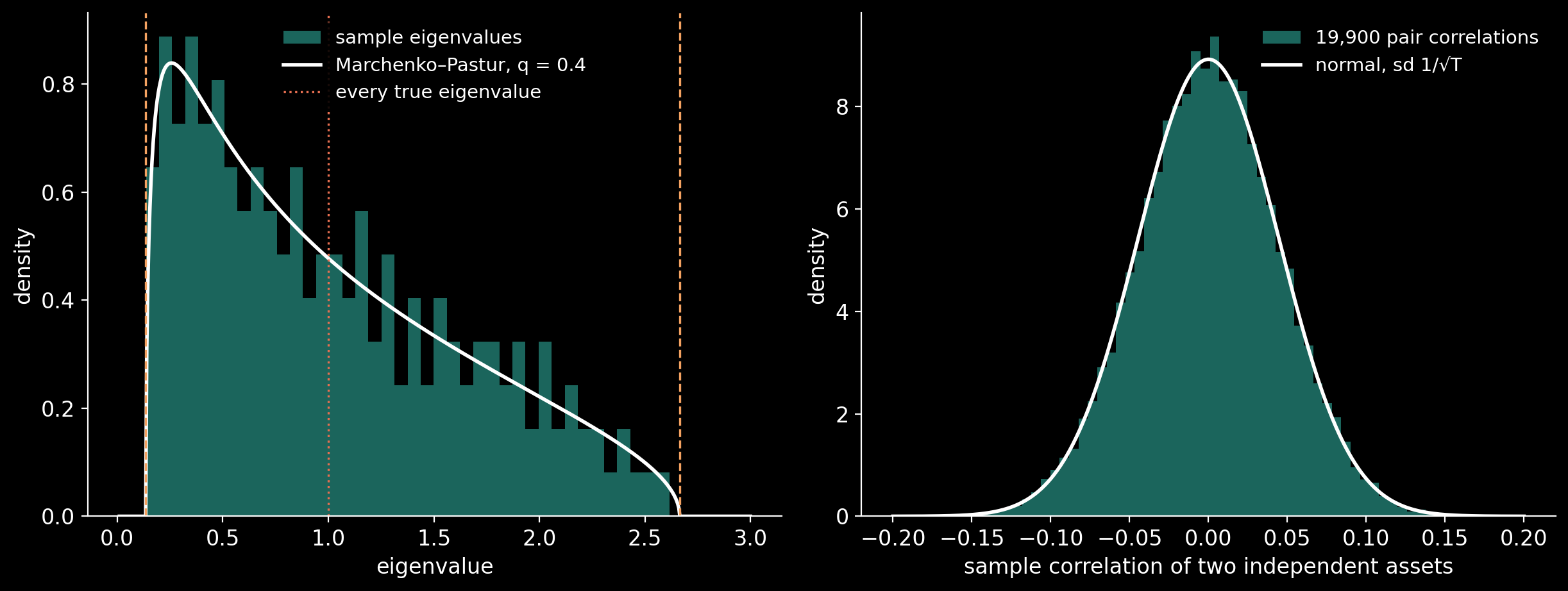
Two hundred assets, five hundred days, every return independent with unit variance. The ratio $q = N/T = 0.4$ sets the band in which the eigenvalues of the sample correlation matrix must fall, and the density inside it:
The true correlation matrix here is the identity: every true eigenvalue is exactly 1.
Two Hundred Independent Assets
import numpy as np

N, T = 200, 500                       # assets, days
q = N / T
rng = np.random.default_rng(1967)     # the year of Marchenko and Pastur
X = rng.standard_normal((T, N))       # independent returns, unit variance
C = np.corrcoef(X, rowvar=False)      # the sample correlation matrix
lam = np.linalg.eigvalsh(C)
lo, hi = (1 - np.sqrt(q)) ** 2, (1 + np.sqrt(q)) ** 2
outside = np.sum((lam < lo) | (lam > hi))

print(f"q = N/T = {q}")
print(f"Marchenko-Pastur band: {lo:.4f} to {hi:.4f}")
print(f"sample eigenvalues:    {lam.min():.4f} to {lam.max():.4f}")
print(f"eigenvalues outside the band: {outside} of {N}")

# q = N/T = 0.4
# Marchenko-Pastur band: 0.1351 to 2.6649
# sample eigenvalues:    0.1362 to 2.6158
# eigenvalues outside the band: 0 of 200
Every true eigenvalue is 1, yet the sample ones run from about a seventh of that to more than two and a half times it. The same noise shows up pair by pair: a sample correlation between two independent series has a standard deviation of about $1/\sqrt{T}$, and with 19,900 pairs some of them are bound to look large.
The Largest Correlation Between Independent Assets
iu = np.triu_indices(N, k=1)
r = C[iu]                             # every pair, once
print(f"pairs: {r.size}")
print(f"spread of the pair correlations: {r.std():.4f}")
print(f"theory, 1/sqrt(T):               {1 / np.sqrt(T):.4f}")
print(f"the largest |correlation|: {np.abs(r).max():.4f}")
print(f"pairs beyond 0.1 either way: {np.sum(np.abs(r) > 0.1)}")

# pairs: 19900
# spread of the pair correlations: 0.0447
# theory, 1/sqrt(T):               0.0447
# the largest |correlation|: 0.1853
# pairs beyond 0.1 either way: 513
A Market With Sectors
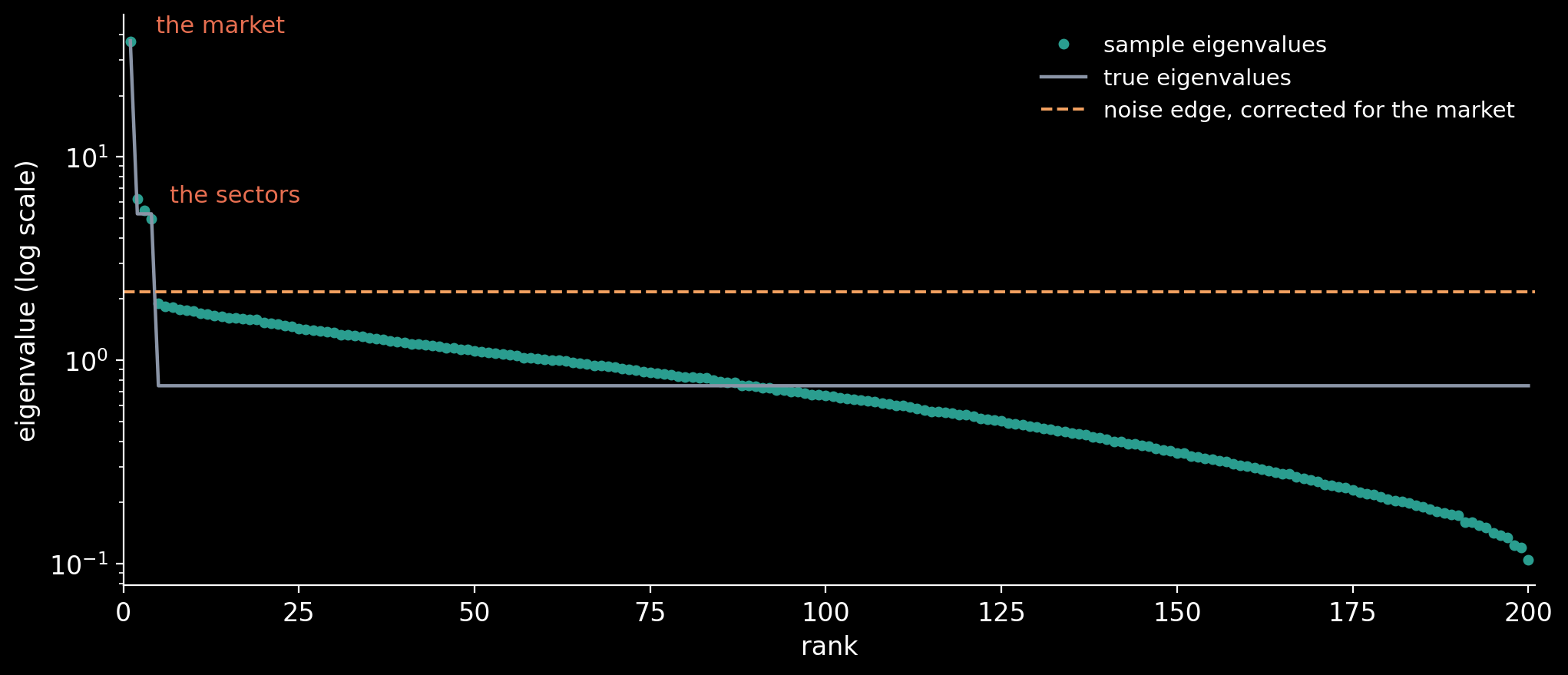
Now plant structure. Every asset loads 0.4 on one market factor, and each belongs to one of four sectors that adds a loading of 0.3 on its own factor; the rest is independent noise, so every asset still has unit variance. The true correlation matrix has exactly four eigenvalues above the rest: one for the market and three that tell the sectors apart. The question is whether the sample matrix shows four.
The edge of the noise band must first be corrected for the market, which carries a share of the total variance (Laloux and co-authors, 1999): the variance left for the noise is $\sigma^2 = 1 – \lambda_{\max}/N$, and the edge becomes $\sigma^2 (1 + \sqrt{q})^2$.
Planting a Market and Four Sectors
beta, gamma, K = 0.4, 0.3, 4          # market loading, sector loading, sectors
sector = np.arange(N) % K
idio = np.sqrt(1 - beta**2 - gamma**2)
m = rng.standard_normal((T, 1))
s = rng.standard_normal((T, K))
R = beta * m + gamma * s[:, sector] + idio * rng.standard_normal((T, N))

C_true = beta**2 + gamma**2 * (sector[:, None] == sector[None, :])
np.fill_diagonal(C_true, 1.0)
C_s = np.corrcoef(R, rowvar=False)
lam_t = np.linalg.eigvalsh(C_true)[::-1]
lam_s = np.linalg.eigvalsh(C_s)[::-1]
sigma2 = 1 - lam_s[0] / N             # the noise variance left after the market
edge = sigma2 * (1 + np.sqrt(q)) ** 2

show = lambda v: ", ".join(f"{x:.2f}" for x in v)
print(f"top true eigenvalues:   {show(lam_t[:6])}")
print(f"top sample eigenvalues: {show(lam_s[:6])}")
print(f"noise edge after the market: {edge:.4f}")
print(f"sample eigenvalues above it: {np.sum(lam_s > edge)}")

# top true eigenvalues:   37.25, 5.25, 5.25, 5.25, 0.75, 0.75
# top sample eigenvalues: 37.02, 6.24, 5.45, 4.97, 1.91, 1.83
# noise edge after the market: 2.1716
# sample eigenvalues above it: 4
Cleaning by Clipping
The simplest cure keeps what rises above the band and treats the rest as noise: the eigenvalues above the edge stay, every eigenvalue inside the band is replaced by their average so the trace stays the same, and the matrix is rebuilt and rescaled back to a correlation matrix (Laloux, Cizeau, Bouchaud and Potters, 1999). Because the truth is known here, the cleaning can be judged directly.
Eigenvalue Clipping
def clip(C, edge):
    w, V = np.linalg.eigh(C)
    noise = w <= edge
    w = w.copy()
    w[noise] = w[noise].mean()        # the bulk flattened, the trace kept
    Cc = (V * w) @ V.T
    d = np.sqrt(np.diag(Cc))
    return Cc / np.outer(d, d)        # back to a correlation matrix

C_c = clip(C_s, edge)
err = lambda A: np.linalg.norm(A - C_true) / np.linalg.norm(C_true)
print(f"distance to the truth, sample:  {err(C_s):.4f}")
print(f"distance to the truth, cleaned: {err(C_c):.4f}")

# distance to the truth, sample:  0.2075
# distance to the truth, cleaned: 0.1159
The Risk It Promises, and the Risk It Delivers
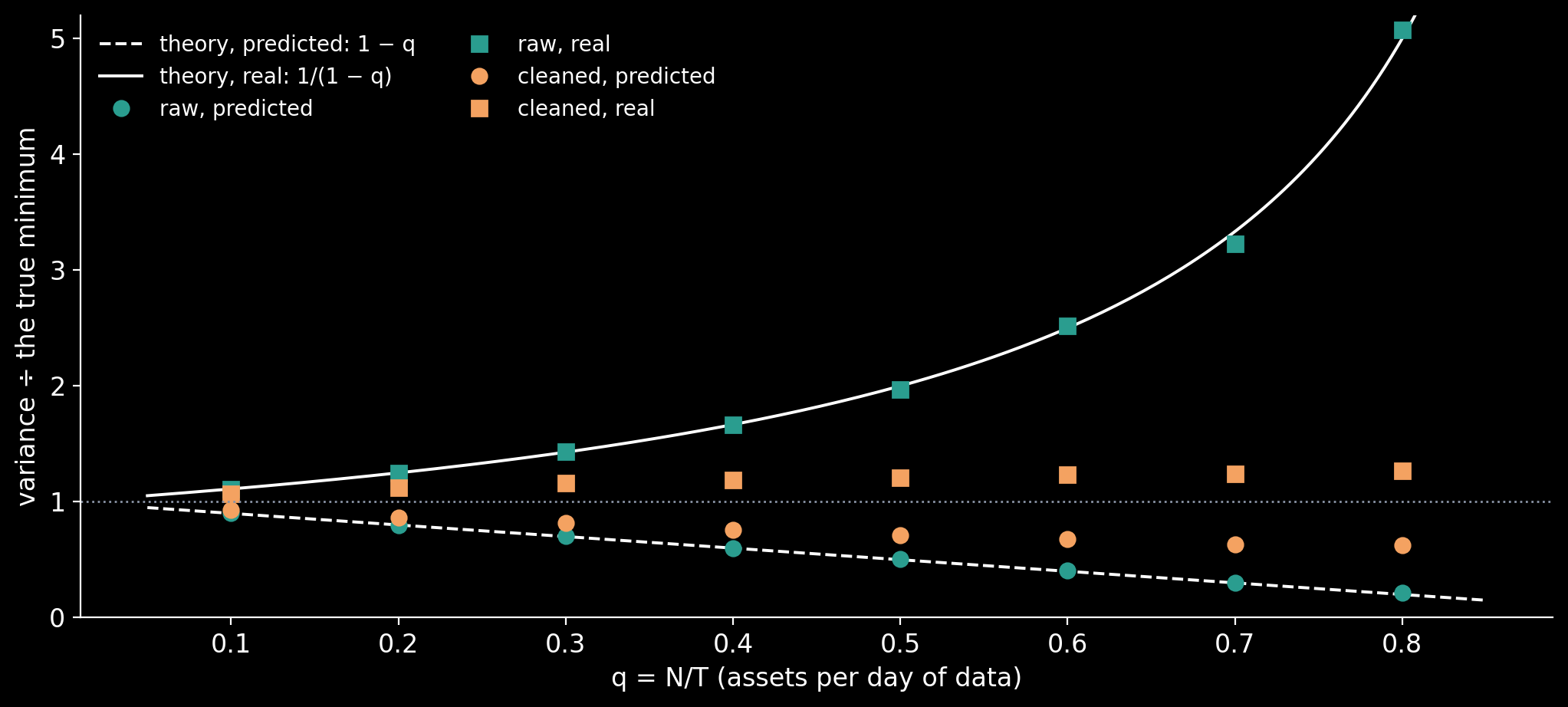
A minimum-variance portfolio weights the assets by $w \propto C^{-1}\mathbf{1}$, and the inverse amplifies the smallest eigenvalues, which are the noisiest. Its predicted variance is computed with the matrix it was built from; its real variance with the truth. For Gaussian returns the theory is exact in the limit: built on the raw sample covariance, the predicted variance is $(1-q)$ times the true minimum and the real one is $1/(1-q)$ times it (Pafka and Kondor, 2003). The portfolio believes it is safer than the best possible portfolio, and is in fact riskier.
Two hundred fresh samples are drawn from the planted market. Each builds a raw portfolio and a cleaned one, and each is scored both ways.
Two Hundred Portfolios, Raw and Cleaned
Lc = np.linalg.cholesky(C_true)
one = np.ones(N)
best = 1 / (one @ np.linalg.solve(C_true, one))   # the true minimum

def minvar(S):
    w = np.linalg.solve(S, one)
    return w / w.sum()

score = {"raw": [], "cleaned": []}
for _ in range(200):
    Z = rng.standard_normal((T, N)) @ Lc.T   # a fresh sample from the truth
    S = Z.T @ Z / T                          # its covariance (mean known: 0)
    d = np.sqrt(np.diag(S))
    Cz = S / np.outer(d, d)
    e = (1 - np.linalg.eigvalsh(Cz)[-1] / N) * (1 + np.sqrt(q)) ** 2
    S_c = clip(Cz, e) * np.outer(d, d)       # cleaned; sample vols kept
    for name, M in (("raw", S), ("cleaned", S_c)):
        w = minvar(M)
        score[name].append((w @ M @ w / best, w @ C_true @ w / best))

for name, v in score.items():
    p, r = np.mean(v, axis=0)
    print(f"{name:8s} predicted {p:.3f} x the minimum, real {r:.3f} x")
print(f"theory   predicted {1 - q:.3f} x the minimum, real {1 / (1 - q):.3f} x")

# raw      predicted 0.604 x the minimum, real 1.656 x
# cleaned  predicted 0.765 x the minimum, real 1.183 x
# theory   predicted 0.600 x the minimum, real 1.667 x
Linear Shrinkage, and Why the Target Matters
A reader on Kaggle, Arhan Canli, asked the question most people would: how does clipping compare with Ledoit–Wolf shrinkage, the estimator most practitioners reach for first? Linear shrinkage pulls the sample covariance $S$ towards a simpler target $F$,
with the intensity $\delta$ estimated from the data to minimise the expected error (Ledoit and Wolf, 2003 and 2004). How well it does depends on the target, and he named the ones worth trying: the scaled identity, which is what most libraries use; one correlation shared by every pair; and a single market factor, here the equally weighted average.
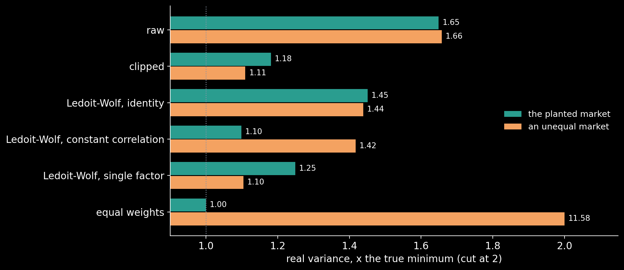
The planted market above has a property that matters for this comparison: every asset has the same loadings and the four sectors are the same size, so the true minimum-variance portfolio is simply the equally weighted one. Any method that pulls the weights towards equal is flattered by it. So the comparison is run on that market and on an unequal one, with market loadings between 0.15 and 0.65, sector loadings up to 0.45, sectors of 80, 60, 40 and 20 assets, and volatilities that differ from asset to asset.
Three Linear Targets Against Clipping
def lw_identity(X):
    # towards the scaled identity, as scikit-learn's LedoitWolf (2004)
    T, N = X.shape
    S = X.T @ X / T
    F = np.trace(S) / N * np.eye(N)
    d2 = np.sum((S - F) ** 2) / N
    b2 = np.sum((X**2).T @ (X**2) / T - S**2) / (N * T)
    delta = min(b2, d2) / d2
    return delta * F + (1 - delta) * S, delta

def lw_constant_correlation(X):
    # towards one correlation for every pair (Ledoit and Wolf, 2004)
    T, N = X.shape
    S = X.T @ X / T
    s = np.sqrt(np.diag(S))
    rbar = (np.sum(S / np.outer(s, s)) - N) / (N * (N - 1))
    F = rbar * np.outer(s, s)
    np.fill_diagonal(F, np.diag(S))
    pi = (X**2).T @ (X**2) / T - S**2
    theta = (X**3).T @ X / T - np.diag(S)[:, None] * S
    off = np.outer(1 / s, s) * theta
    np.fill_diagonal(off, 0)
    rho = np.trace(pi) + rbar * off.sum()
    kappa = (pi.sum() - rho) / np.sum((F - S) ** 2)
    delta = max(0.0, min(1.0, kappa / T))
    return delta * F + (1 - delta) * S, delta

def lw_single_factor(X):
    # towards one market factor, the equally weighted average (2003)
    T, N = X.shape
    S = X.T @ X / T
    m = X.mean(axis=1)
    c, vm = X.T @ m / T, m @ m / T
    F = np.outer(c, c) / vm
    np.fill_diagonal(F, np.diag(S))
    y, z = X**2, X * m[:, None]
    p = np.sum(y.T @ y / T) - np.sum(S**2)
    r_diag = np.sum(y**2) / T - np.sum(np.diag(S) ** 2)
    v1 = y.T @ z / T - c[:, None] * S
    r1 = (np.sum(v1 * c[None, :]) - np.sum(np.diag(v1) * c)) / vm
    v3 = z.T @ z / T - vm * S
    r3 = (np.sum(v3 * np.outer(c, c)) - np.sum(np.diag(v3) * c**2)) / vm**2
    kappa = (p - (r_diag + 2 * r1 - r3)) / np.sum((S - F) ** 2)
    delta = max(0.0, min(1.0, kappa / T))
    return delta * F + (1 - delta) * S, delta

def unequal_market(g):
    sec = np.repeat(np.arange(4), [80, 60, 40, 20])
    b = g.uniform(0.15, 0.65, N)
    c = np.minimum(g.uniform(0.0, 0.45, N), np.sqrt(0.9 - b**2))
    corr = np.outer(b, b) + np.outer(c, c) * (sec[:, None] == sec[None, :])
    np.fill_diagonal(corr, 1.0)
    vol = np.exp(g.normal(0, 0.35, N))
    return corr * np.outer(vol, vol)

g = np.random.default_rng(2004)
MARKETS = {"the planted market": C_true, "an unequal market": unequal_market(g)}
LINEAR = {"Ledoit-Wolf, identity": lw_identity,
          "Ledoit-Wolf, constant correlation": lw_constant_correlation,
          "Ledoit-Wolf, single factor": lw_single_factor}
METHODS = ["raw", "clipped", *LINEAR, "equal weights"]
table, intensity = {}, {}
for mname, Sig in MARKETS.items():
    L_ = np.linalg.cholesky(Sig)
    floor = 1 / (one @ np.linalg.solve(Sig, one))      # the true minimum
    acc = {k: [] for k in METHODS}
    dl = {k: [] for k in LINEAR}
    for _ in range(100):
        Z = g.standard_normal((T, N)) @ L_.T
        S = Z.T @ Z / T
        d = np.sqrt(np.diag(S))
        Cz = S / np.outer(d, d)
        e = (1 - np.linalg.eigvalsh(Cz)[-1] / N) * (1 + np.sqrt(q)) ** 2
        est = {"raw": S, "clipped": clip(Cz, e) * np.outer(d, d)}
        for k, f in LINEAR.items():
            est[k], delta = f(Z)
            dl[k].append(delta)
        for k, M in est.items():
            w = minvar(M)
            acc[k].append((w @ M @ w / floor, w @ Sig @ w / floor))
        acc["equal weights"].append((np.nan, (one @ Sig @ one) / N**2 / floor))
    table[mname] = {k: np.mean(v, axis=0) for k, v in acc.items()}
    intensity[mname] = {k: np.mean(v) for k, v in dl.items()}

print(f"{'variance, x the true minimum':34s}{'planted market':>20s}"
      f"{'unequal market':>20s}")
print(f"{'':34s}{'predicted':>10s}{'real':>10s}{'predicted':>10s}{'real':>10s}")
for k in METHODS:
    a, b = table["the planted market"][k], table["an unequal market"][k]
    cell = lambda x: f"{'-':>10s}" if np.isnan(x) else f"{x:10.3f}"
    print(f"{k:34s}{cell(a[0])}{a[1]:10.3f}{cell(b[0])}{b[1]:10.3f}")
print()
for k in LINEAR:
    print(f"fitted intensity, {k[13:]:22s}: planted "
          f"{intensity['the planted market'][k]:.3f}, "
          f"unequal {intensity['an unequal market'][k]:.3f}")

# variance, x the true minimum            planted market      unequal market
#                                    predicted      real predicted      real
# raw                                    0.600     1.649     0.606     1.658
# clipped                                0.759     1.181     1.063     1.110
# Ledoit-Wolf, identity                  0.608     1.451     0.765     1.439
# Ledoit-Wolf, constant correlation      0.887     1.099     1.086     1.418
# Ledoit-Wolf, single factor             0.705     1.249     0.939     1.105
# equal weights                              -     1.000         -    11.581
#
# fitted intensity, identity              : planted 0.058, unequal 0.055
# fitted intensity, constant correlation  : planted 0.589, unequal 0.221
# fitted intensity, single factor         : planted 0.466, unequal 0.631
An Empirical Band for Real Returns
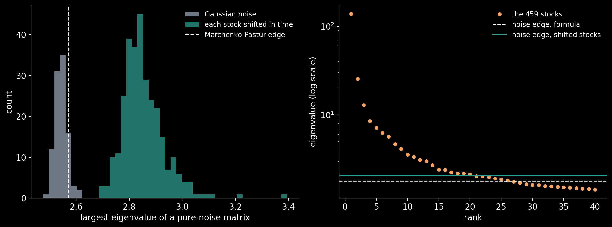
The Marchenko–Pastur band assumes returns that are independent from day to day and light-tailed. Real returns are neither: they have fat tails and their volatility comes in clusters, and both widen the band that noise fills, so a few eigenvalues just above the formula’s edge can still be noise. The reader’s second suggestion measures how far the edge moves for a given dataset: keep each asset’s own series, with its tails and its clustering, but shift it in time by a random circular lag, independently of every other asset. That breaks every link between the assets and nothing else, and the largest eigenvalue of many such shuffles is an empirical edge.
The returns are daily closing prices of the S&P 500 members from 8 February 2013 to 7 February 2018, from a public-domain Kaggle dataset: 470 stocks have a price on every one of the 1,259 days. The prices are not adjusted for splits and spin-offs, so a stock is dropped if it has a one-day move by a factor of more than 1.75, or a move of more than 20% that reverses by more than 20% the next day, which is a bad print; that removes 11 and leaves 459. The saved file holds their 1,258 daily log returns.
Shifting Each Stock in Time
import pandas as pd
rets = pd.read_csv("data/sp500_returns.csv", index_col="date")
Xr = ((rets - rets.mean()) / rets.std()).to_numpy()
Tr, Nr = Xr.shape
qr = Nr / Tr
lam_r = np.linalg.eigvalsh(Xr.T @ Xr / Tr)[::-1]
edge_mp = (1 + np.sqrt(qr)) ** 2
noise_share = 1 - lam_r[0] / Nr          # the variance left after the market

g = np.random.default_rng(1999)
shifted, gaussian = [], []
for _ in range(300):
    Xs = np.column_stack([np.roll(Xr[:, j], g.integers(Tr))
                          for j in range(Nr)])
    shifted.append(np.linalg.eigvalsh(Xs.T @ Xs / Tr)[-1])
for _ in range(100):
    Zg = g.standard_normal((Tr, Nr))
    Zg = (Zg - Zg.mean(0)) / Zg.std(0)
    gaussian.append(np.linalg.eigvalsh(Zg.T @ Zg / Tr)[-1])
shifted, gaussian = np.array(shifted), np.array(gaussian)
edge_emp = np.quantile(shifted, 0.95)

print(f"{Nr} stocks, {Tr} days, q = {qr:.3f}; excess kurtosis, median stock "
      f"{rets.kurt().median():.2f}")
print(f"largest eigenvalue of pure noise: Marchenko-Pastur edge {edge_mp:.4f}")
print(f"  Gaussian noise, same size:   median {np.median(gaussian):.4f}, "
      f"95th percentile {np.quantile(gaussian, 0.95):.4f}")
print(f"  each stock shifted in time:  median {np.median(shifted):.4f}, "
      f"95th percentile {edge_emp:.4f}")
print(f"the market's eigenvalue {lam_r[0]:.2f}; the noise keeps {noise_share:.1%} "
      f"of the variance")
for name, e in (("Marchenko-Pastur", edge_mp),
                ("shifted, 95th percentile", edge_emp)):
    print(f"eigenvalues above the {name} edge after the market "
          f"({noise_share * e:.4f}): {np.sum(lam_r > noise_share * e)}")

# 459 stocks, 1258 days, q = 0.365; excess kurtosis, median stock 5.66
# largest eigenvalue of pure noise: Marchenko-Pastur edge 2.5729
#   Gaussian noise, same size:   median 2.5419, 95th percentile 2.5720
#   each stock shifted in time:  median 2.8393, 95th percentile 2.9953
# the market's eigenvalue 138.48; the noise keeps 69.8% of the variance
# eigenvalues above the Marchenko-Pastur edge after the market (1.7967): 26
# eigenvalues above the shifted, 95th percentile edge after the market (2.0916): 20
What the Noise Costs
With 200 assets and 500 days, all but four of the 200 eigenvalues of the planted market’s sample matrix sit in the band that pure noise would fill. A portfolio built on the raw matrix promises a variance 40% below the true minimum and delivers one 66% above it: 0.604 and 1.656 times the minimum, against 0.600 and 1.667 from the theory, written down before a single number is drawn. Clipping the band costs a few lines of code and brings the real variance down to 18% above the minimum. It does not create information, though: it only stops the optimiser from trading on noise.
Linear shrinkage does as well as its target. Towards the scaled identity, the target most libraries use, Ledoit–Wolf moves the matrix by under 6% and the portfolio delivers 1.44 to 1.45 times the minimum on both markets. Towards one correlation for every pair it beats clipping on the planted market, 1.10 against 1.18, but only because the truth there is close to that target and the best portfolio is equal weights; on the unequal market it falls back to 1.42. Towards a single market factor it is level with clipping on the unequal market, 1.105 against 1.110. Clipping needs no target, which is its advantage when nobody knows the right one.
On real returns the band itself moves. For 459 S&P 500 stocks over five years, shifting each stock in time breaks every link between them but keeps its fat tails and clustered volatility, and the largest eigenvalue of that noise is 2.84 at the median and 3.00 at the 95th percentile, against 2.57 from the formula and from Gaussian noise of the same size. After the market, the formula counts 26 eigenvalues above the noise and the empirical edge 20: six that the formula would call structure are within reach of noise.
Sources
- V. A. Marčenko and L. A. Pastur, “Distribution of eigenvalues for some sets of random matrices”, Mathematics of the USSR-Sbornik 1 (1967) 457–483.
- L. Laloux, P. Cizeau, J.-P. Bouchaud and M. Potters, “Noise dressing of financial correlation matrices”, Physical Review Letters 83 (1999) 1467–1470.
- V. Plerou, P. Gopikrishnan, B. Rosenow, L. A. N. Amaral and H. E. Stanley, “Universal and nonuniversal properties of cross correlations in financial time series”, Physical Review Letters 83 (1999) 1471–1474.
- S. Pafka and I. Kondor, “Noisy covariance matrices and portfolio optimization II”, Physica A 319 (2003) 487–494.
- J. Bun, J.-P. Bouchaud and M. Potters, “Cleaning large correlation matrices: tools from random matrix theory”, Physics Reports 666 (2017) 1–109.
- O. Ledoit and M. Wolf, “Improved estimation of the covariance matrix of stock returns with an application to portfolio selection”, Journal of Empirical Finance 10 (2003) 603–621.
- O. Ledoit and M. Wolf, “A well-conditioned estimator for large-dimensional covariance matrices”, Journal of Multivariate Analysis 88 (2004) 365–411.
- O. Ledoit and M. Wolf, “Honey, I shrunk the sample covariance matrix”, The Journal of Portfolio Management 30(4) (2004) 110–119.
- C. Nugent, “S&P 500 stock data”, Kaggle dataset camnugent/sandp500, CC0: Public Domain.
Working on a pricing model or risk system? Let’s talk.