
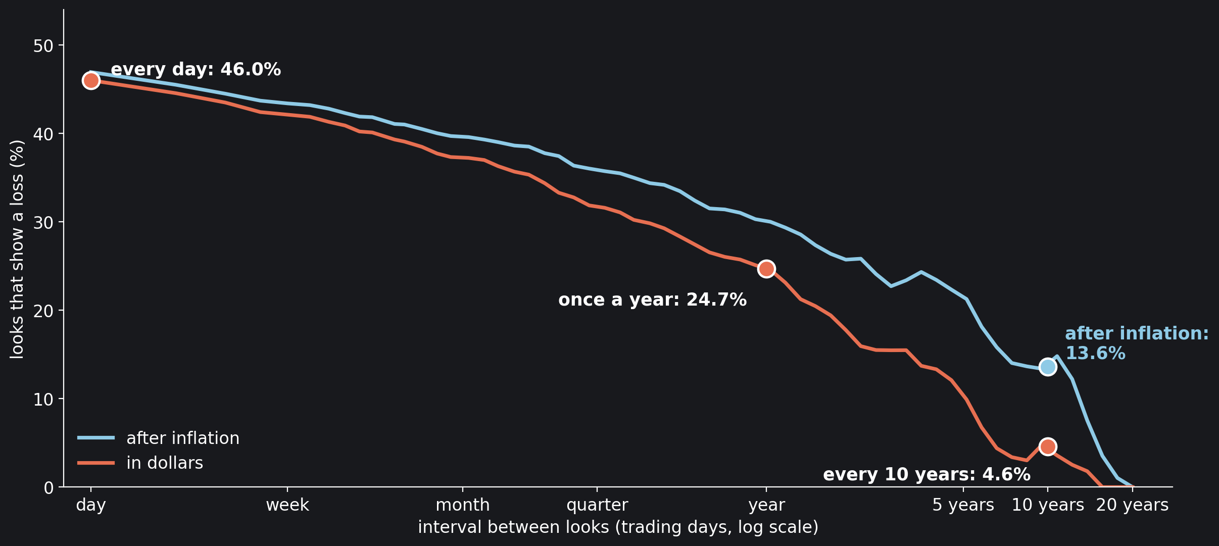
Two people own the same fund: the S&P 500, with every dividend reinvested. One opens the account every evening. The other looks once a year, when the annual statement comes. Over the 98 years since January 1928 the fund did the same thing for both of them and turned each dollar into 14,790. What they saw was not the same. The daily looker saw a loss on 46.0% of the days he looked; the yearly one in about a quarter of the years.
That matters because a loss does not feel like a gain of the same size. In their 1992 update of prospect theory, Amos Tversky and Daniel Kahneman put a number on the difference, the coefficient of loss aversion λ, and estimated it at 2.25: a loss weighs about two and a quarter times an equal gain. Three years later Shlomo Benartzi and Richard Thaler joined the two facts. They called the combination of loss aversion and frequent looking myopic loss aversion, and offered it as the answer to the equity premium puzzle, “the empirical fact that stocks have outperformed bonds over the last century by a surprisingly large margin.” With Tversky and Kahneman’s parameters, they found, the size of that margin fits “if investors evaluate their portfolios annually.”
This notebook measures both halves of the argument on 24,804 trading days of the S&P 500, from January 1928 to October 2026, and on a 10-year bond, month by month: how often a look shows a loss, from a look a day to one every twenty years; how far apart the looks must be before a loss-averse investor feels them as gains; and, with Benartzi and Thaler’s own model and parameters, how often he can look and still prefer stocks to bonds. An earlier notebook here, The Bet Samuelson’s Colleague Refused, measured the break-even against holding nothing; this one adds the comparison Benartzi and Thaler actually made, stocks against bonds, and runs it to 2026.
Key findings
- A daily look at the S&P 500 with dividends showed a loss on 46.0% of days, a yearly look in 24.7% of years and a ten-year look 4.6% of the time.
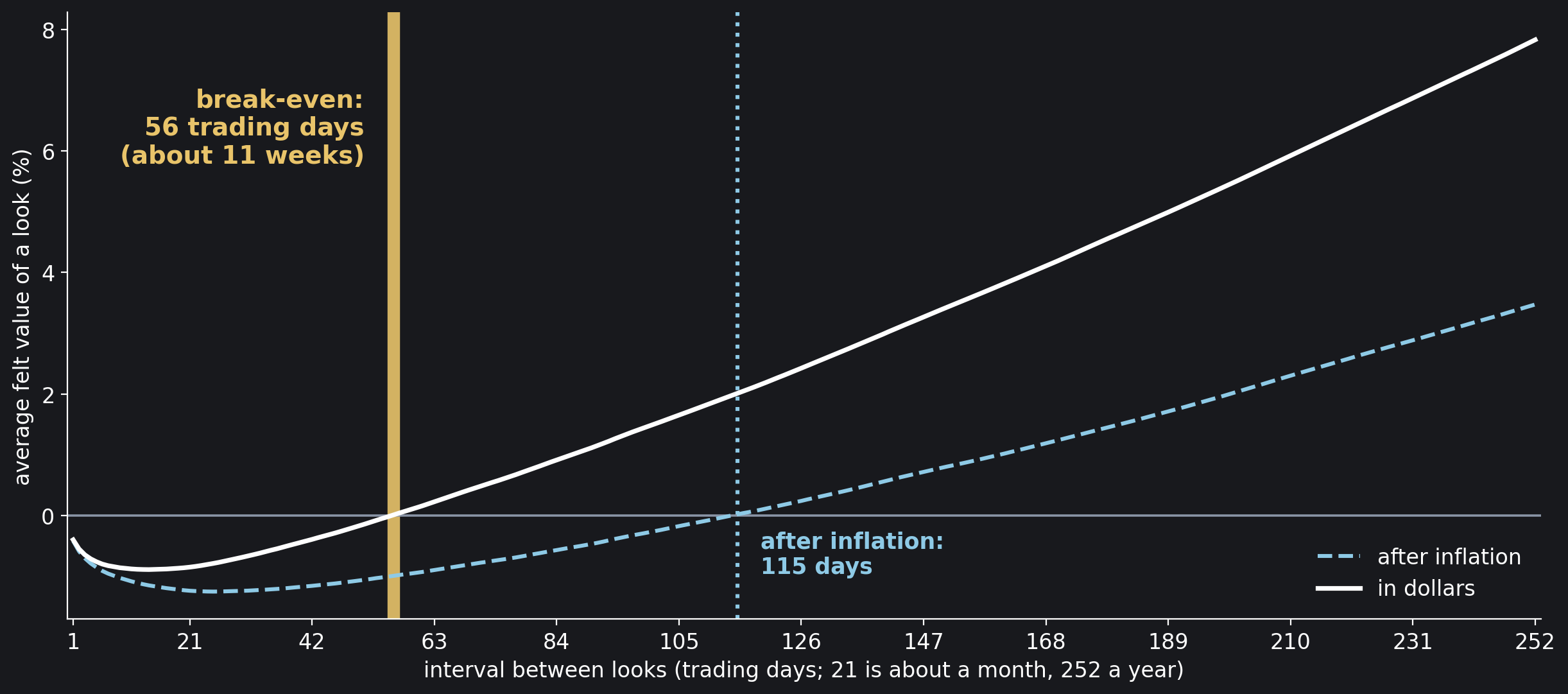
- With a loss weighing 2.25 times an equal gain, the daily look is a net pain on average; the felt value turns positive, and stays positive, only when the looks are at least 56 trading days apart, about eleven weeks.
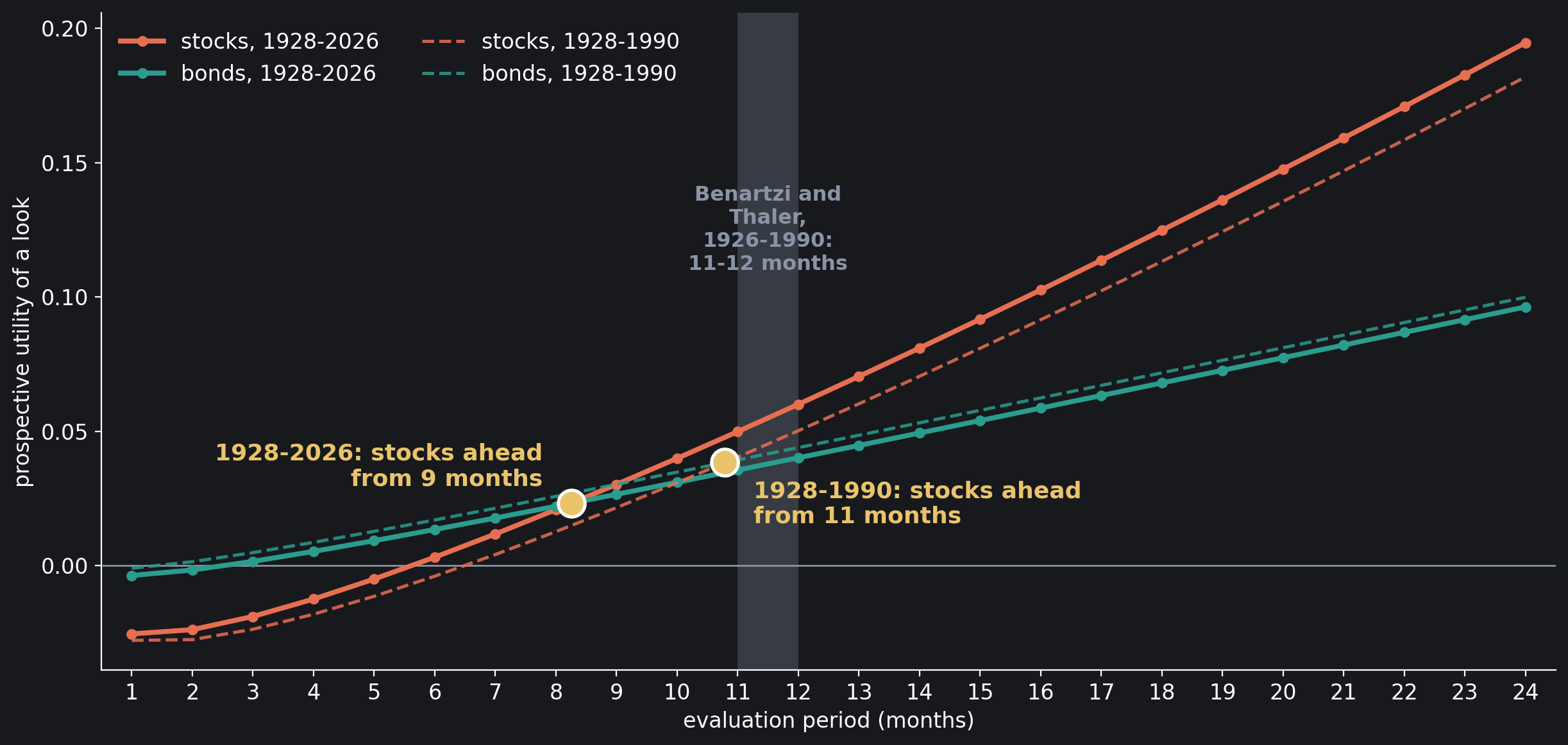
- Benartzi and Thaler’s stocks-against-bonds model, rebuilt with their parameters, puts stocks ahead of bonds from an evaluation period of 11 months on 1928–1990 (theirs, on 1926–1990: 11 to 12 months) and from 9 months on 1928–2026.
- That 9 rests on drawing months independently, as they did: kept in history’s order, the same months put stocks ahead only from 18 months.
- After inflation the long look comforts less: a ten-year look showed a loss 13.6% of the time, three times the 4.6% in dollars, and the break-even doubles to 115 trading days.
Two Investors, One Fund
The data file holds one row per trading day: the day’s total return, which is the change in the S&P 500’s closing price plus one trading day’s share of the year’s dividend from Robert Shiller’s monthly series, and Shiller’s consumer price index for the month. The closes are Yahoo Finance prices from a public-domain Kaggle dataset. A look is a window of $h$ consecutive trading days, and every window in the 98 years counts, starting on any day, so the windows overlap.
Two Investors, One Fund
import numpy as np
import pandas as pd

df = pd.read_csv("data/sp500_total_return_daily.csv", index_col="date",
                 parse_dates=True)
r = df["total_return"].to_numpy()      # simple daily return, dividends in
lg = np.log1p(r)                       # daily log return
L = np.r_[0.0, np.cumsum(lg)]          # log wealth, one entry per close
DAYS = 252                             # trading days in a year
print(f"{len(r):,} trading days, {df.index[0]:%d %b %Y} to "
      f"{df.index[-1]:%d %b %Y}")
print(f"one dollar, dividends reinvested, became {np.exp(L[-1]):,.0f}")

def returns_over(h, logw=L):           # every window of h trading days
    return np.expm1(logw[h:] - logw[:-h])

for name, h in (("every day", 1), ("once a year", DAYS)):
    R = returns_over(h)
    print(f"looking {name:<12}{len(R):>7,} possible looks, "
          f"{np.mean(R < 0):.1%} show a loss")

# 24,804 trading days, 03 Jan 1928 to 01 Oct 2026
# one dollar, dividends reinvested, became 14,790
# looking every day    24,804 possible looks, 46.0% show a loss
# looking once a year  24,553 possible looks, 24.7% show a loss
A dollar invested in January 1928 became 14,790 with every dividend reinvested. Of the 24,804 daily looks, 46.0% showed a loss; of the 24,553 possible yearly looks, a year being 252 trading days from any starting day, 24.7% did. Same fund, same history: the daily looker sees red almost every other day, the yearly one about one year in four.
How Often a Look Shows a Loss
The cell counts the losing looks at ten intervals, from a day to twenty years, in dollars and after inflation. Shiller’s consumer price index is monthly, so each month’s inflation is spread evenly over its trading days.
How Often a Look Shows a Loss
month = df.index.to_period("M")
cpi = df["cpi"].groupby(month).first()
infl = np.log(cpi).diff().fillna(0.0)      # log inflation of each month
per_day = (infl / month.value_counts()).reindex(month).to_numpy()
Lr = np.r_[0.0, np.cumsum(lg - per_day)]   # log wealth after inflation

LOOKS = {"day": 1, "week": 5, "month": 21, "quarter": 63,
         "half-year": 126, "year": 252, "2 years": 504,
         "5 years": 1260, "10 years": 2520, "20 years": 5040}
print(f"{'look every':<11}{'loss, nominal':>15}{'loss, real':>12}")
for name, h in LOOKS.items():
    print(f"{name:<11}{np.mean(returns_over(h) < 0):>15.1%}"
          f"{np.mean(returns_over(h, Lr) < 0):>12.1%}")

# look every   loss, nominal  loss, real
# day                  46.0%       46.9%
# week                 42.1%       43.4%
# month                37.2%       39.6%
# quarter              31.9%       35.8%
# half-year            28.4%       33.4%
# year                 24.7%       29.9%
# 2 years              17.0%       25.7%
# 5 years              10.5%       21.8%
# 10 years              4.6%       13.6%
# 20 years              0.0%        0.0%
In dollars the share falls steadily with the interval: 42.1% for a weekly look, 37.2% monthly, 31.9% quarterly, 24.7% yearly, 10.5% every five years and 4.6% every ten. No twenty-year window since 1928 ended below its start, but the windows overlap and fewer than five separate twenty-year spans fit in 98 years, so that 0.0% rests on a handful of independent stretches. After inflation every share is higher; Figure 1 shows both curves, and the section After Inflation comes back to them.
How a Look Feels
Score the return $R$ of each look the way a loss-averse investor feels it, a gain at face value and a loss $\lambda$ times as heavy, with Tversky and Kahneman’s $\lambda = 2.25$,
and average it over every window of the same length. A positive average means the looks, taken together, feel like gains; a negative one means the losses outweigh them, although the money grew. These are straight lines, the simplest form of loss aversion; Benartzi and Thaler’s curved version comes in the next section. The cell scores every interval up to two years, in dollars and after inflation, and finds the break-even: the interval from which the felt value stays above zero.
How a Look Feels
LAM = 2.25                             # a loss weighs 2.25 equal gains

def felt(R, lam=LAM):                  # the average felt value of a look
    return np.where(R >= 0, R, lam * R).mean()

def break_even(v, H):                  # from here on, always above zero
    return H[np.flatnonzero(v < 0)[-1] + 1]

H = np.arange(1, 505)                  # every interval up to two years
F = np.array([felt(returns_over(h)) for h in H])
Fr = np.array([felt(returns_over(h, Lr)) for h in H])
print(f"{'look every':<11}{'felt, nominal':>15}{'felt, real':>12}")
for name in ("day", "week", "month", "quarter", "half-year", "year"):
    h = LOOKS[name]
    print(f"{name:<11}{F[h - 1]:>+15.2%}{Fr[h - 1]:>+12.2%}")
T_be, T_real = break_even(F, H), break_even(Fr, H)
print(f"\nworst interval: {H[F.argmin()]} trading days, {F.min():+.2%}")
print(f"break-even: {T_be} trading days ({T_be / 5:.1f} weeks) nominal, "
      f"{T_real} ({T_real / 5:.1f} weeks) after inflation")

# look every   felt, nominal  felt, real
# day                 -0.40%      -0.42%
# week                -0.76%      -0.86%
# month               -0.85%      -1.24%
# quarter             +0.22%      -0.90%
# half-year           +2.42%      +0.24%
# year                +7.83%      +3.47%
#
# worst interval: 14 trading days, -0.89%
# break-even: 56 trading days (11.2 weeks) nominal, 115 (23.0 weeks) after inflation
Looked at every day, the S&P 500 feels like a loss, −0.40% of the account per look on average, and the feeling gets worse before it gets better: −0.76% for a weekly look, −0.85% for a monthly one, worst at 14 trading days, −0.89%. The typical loss grows with the square root of the interval while the drift grows in proportion to it, and at first the square root wins. From 56 trading days on, about eleven weeks, the felt value is positive and stays there: +0.22% for a quarterly look, +2.42% for a half-yearly one and +7.83% for a yearly one. Figure 2 marks the break-even.
Benartzi and Thaler’s Comparison
The break-even above sets stocks against holding nothing. Benartzi and Thaler set them against bonds, the choice an investor actually makes, and used Tversky and Kahneman’s full cumulative prospect theory rather than straight lines. Their parameters, as their paper states them (the working paper of 1993, pages 9 and 10): a gain $x$ is valued at $x^\alpha$ and a loss at $-\lambda(-x)^\beta$, and “They have estimated α and β to be 0.88 and λ to be 2.25.” Probabilities are bent as well. Each outcome’s decision weight is $w(P_i) – w(P_i^*)$, where $P_i$ is the chance of an outcome at least as good as it and $P_i^*$ the chance of one strictly better, “applied separately for gains and losses” (for a loss, read as bad and strictly worse), with
and γ estimated “to be .61 in the domain of gains and .69 in the domain of losses.” With γ below 1 the rare outcomes at either end weigh more than their chance. The prospective utility of an asset is the sum, over its outcomes, of value times decision weight.
Their returns were monthly, from CRSP, 1926 to 1990: the CRSP stock index against 5-year bonds. Here the stocks are the S&P 500, month by month from the daily file, and the bond is a 10-year bond priced from the long-term interest rate in Shiller’s monthly data, a column he labels GS10, the name of the Federal Reserve’s 10-year Treasury yield. His workbook carries a monthly total return for that bond, and the column matches, in every month, a bond bought at par at month $t$’s long-term yield $y_t$, paying $y_t/12$ a month, and sold a month later, with 119 months still to run, at month $t+1$’s yield:
Before April 1953 the workbook’s yield moves in equal steps from one January to the next, an annual series spread over the months, so the bond’s monthly returns are smoother there than a traded bond’s would have been. The cell checks the formula against the file and sets the two assets side by side.
Stocks and Bonds, Month by Month
mo = pd.Series(lg, index=df.index).groupby(month).sum()
stocks = np.expm1(mo).loc[:"2026-09"]  # October 2026 has one day only
bd = pd.read_csv("data/shiller_bond_monthly.csv", index_col="month")
bonds = bd["bond_return"].dropna()     # month t's yield to month t+1's

y = bd["gs10"].to_numpy() / 100        # the yield, as a fraction
y0, y1 = y[:-1], y[1:]
k = (1 + y1 / 12) ** -119              # 119 months still to run
sold = y0 / y1 * (1 - k) + k           # the bond's price a month later
gap = np.abs(y0 / 12 + sold - 1 - bonds.to_numpy()).max()
print(f"stocks: {len(stocks)} months, {stocks.index[0]} to "
      f"{stocks.index[-1]}")
print(f"bonds:  {len(bonds)} months, {bonds.index[0]} to "
      f"{bonds.index[-1]} (each to the next month)")
print(f"bond formula against the file: largest gap {gap:.10f}")
for name, x in (("stocks", stocks), ("bonds", bonds)):
    print(f"{name:<7} mean {x.mean() * 12:6.2%} a year, spread "
          f"{x.std() * np.sqrt(12):6.2%}, months that lost "
          f"{np.mean(x < 0):.1%}")

# stocks: 1185 months, 1928-01 to 2026-09
# bonds:  1185 months, 1927-12 to 2026-08 (each to the next month)
# bond formula against the file: largest gap 0.0000000000
# stocks  mean 11.47% a year, spread 18.52%, months that lost 37.4%
# bonds   mean  4.75% a year, spread  5.55%, months that lost 30.1%
The formula gives back the file’s bond return in all 1,185 months. Over those months stocks returned 11.47% a year on average with a yearly spread of 18.52%, the bond 4.75% with 5.55%; stocks lost money in 37.4% of months, the bond in 30.1%.
Then Benartzi and Thaler drew: “distributions of returns are generated for various time horizons by drawing 10,000 n-month returns (with replacement) from the CRSP time series.” The returns were ranked and read at 20 intervals along the distribution, and the prospective utility of each asset computed for evaluation periods of 1 to 18 months. The notebook reads the draw as $n$ months picked independently from the history and compounded, and instead of 10,000 random draws it computes the distribution those draws come from: the distribution of one month’s log return, on a grid of 0.0005, convolved with itself $n$ times. No random number is used and no intervals are needed; Benartzi and Thaler found 100 intervals instead of 20 gave results “substantially the same”. The comparison runs twice, on every month from 1928 to 2026 and on 1928 to 1990, the years closest to theirs.
The Weights
A, LOSS = 0.88, 2.25                   # value: x**A, or -LOSS * (-x)**A
G_GAIN, G_LOSS = 0.61, 0.69            # how probabilities are weighted

def w(p, g):                           # Tversky and Kahneman's weights
    p = np.minimum(p, 1.0)
    return p**g / (p**g + (1 - p)**g) ** (1 / g)

for q in (0.01, 0.05, 0.5):
    print(f"a {q:.0%} chance weighs as {w(q, G_GAIN):.1%} for a gain, "
          f"{w(q, G_LOSS):.1%} for a loss")

# a 1% chance weighs as 5.5% for a gain, 4.0% for a loss
# a 5% chance weighs as 13.2% for a gain, 11.1% for a loss
# a 50% chance weighs as 42.1% for a gain, 45.4% for a loss
Read on cumulative chances, the weighting lifts the ends of the distribution and flattens its middle: the best 1% of outcomes weigh as 5.5% (the worst 1% as 4.0%), the best 5% as 13.2% (the worst as 11.1%), while a 50% chance counts as only 42.1% (45.4%). The next cell builds every $n$-month return with its probability and the prospective utility of a distribution, and checks the grid.
Prospective Utility
STEP = 0.0005                          # grid for monthly log returns

def n_months(x, n):                    # every n-month return made of n
    k = np.round(np.log1p(x) / STEP).astype(int)    # months drawn with
    p1 = np.bincount(k - k.min()) / len(k)          # replacement, and
    p = p1                                          # its probability
    for _ in range(n - 1):
        p = np.convolve(p, p1)
    R = np.expm1((np.arange(len(p)) + n * k.min()) * STEP)
    return R[p > 0], p[p > 0]

def prospect(R, p):                    # cumulative prospect theory
    up, dn = R > 0, R < 0
    Pg = np.cumsum(p[up][::-1])        # chance of a gain at least this
    Pl = np.cumsum(p[dn])              # chance of a loss at least this
    gain = np.diff(np.r_[0, w(Pg, G_GAIN)]) * R[up][::-1] ** A
    loss = np.diff(np.r_[0, w(Pl, G_LOSS)]) * (-R[dn]) ** A
    return gain.sum() - LOSS * loss.sum()

R, p = n_months(stocks.to_numpy(), 12)
print(f"12 months of stocks drawn on the grid: mean {(p * R).sum():.3%}; "
      f"exact: {(1 + stocks.mean()) ** 12 - 1:.3%}")

# 12 months of stocks drawn on the grid: mean 12.094%; exact: 12.093%
The grid costs nothing that shows: twelve months drawn on it have a mean return of 12.094%, against 12.093% exactly. The next cell runs the two functions for evaluation periods of 1 to 24 months, for stocks and for the bond, on both periods, and finds the shortest evaluation period from which stocks stay ahead of the bond.
Stocks Against Bonds
N = np.arange(1, 25)                   # evaluation periods, in months

def utilities(st, bo, value=prospect):
    us = np.array([value(*n_months(st, n)) for n in N])
    ub = np.array([value(*n_months(bo, n)) for n in N])
    return us, ub

def crossing(us, ub):                  # stocks ahead from here on
    return N[np.flatnonzero(us < ub)[-1] + 1]

full = utilities(stocks.to_numpy(), bonds.to_numpy())
old = utilities(stocks[:"1990-12"].to_numpy(), bonds[:"1990-11"].to_numpy())
print(f"{'months':>6}{'1928-2026':>20}{'1928-1990':>20}")
print(f"{'':>6}{'stocks':>10}{'bonds':>10}{'stocks':>10}{'bonds':>10}")
for i in range(18):
    print(f"{N[i]:>6}{full[0][i]:>10.4f}{full[1][i]:>10.4f}"
          f"{old[0][i]:>10.4f}{old[1][i]:>10.4f}")
print(f"\nstocks ahead of bonds from {crossing(*full)} months (1928-2026),"
      f" {crossing(*old)} months (1928-1990)")

# months           1928-2026           1928-1990
#           stocks     bonds    stocks     bonds
#      1   -0.0255   -0.0037   -0.0279   -0.0010
#      2   -0.0239   -0.0017   -0.0276    0.0014
#      3   -0.0190    0.0015   -0.0238    0.0048
#      4   -0.0125    0.0052   -0.0182    0.0086
#      5   -0.0051    0.0092   -0.0115    0.0127
#      6    0.0031    0.0134   -0.0040    0.0170
#      7    0.0117    0.0177    0.0041    0.0213
#      8    0.0208    0.0221    0.0126    0.0257
#      9    0.0302    0.0265    0.0215    0.0302
#     10    0.0399    0.0310    0.0308    0.0348
#     11    0.0499    0.0355    0.0404    0.0393
#     12    0.0600    0.0401    0.0502    0.0439
#     13    0.0704    0.0447    0.0602    0.0485
#     14    0.0810    0.0493    0.0705    0.0531
#     15    0.0917    0.0540    0.0809    0.0578
#     16    0.1026    0.0586    0.0915    0.0624
#     17    0.1137    0.0633    0.1023    0.0671
#     18    0.1248    0.0680    0.1132    0.0717
#
# stocks ahead of bonds from 9 months (1928-2026), 11 months (1928-1990)
Looked at every month, stocks have a prospective utility of −0.0255 and the bond −0.0037: both feel like losses, stocks far more. Both rise with the evaluation period, stocks faster. On 1928–1990 stocks pass the bond at 11 months, inside Benartzi and Thaler’s 11 to 12 months on 1926–1990, from a different index, a different bond and different data: their result reproduces. With the years since 1990 added, stocks pass the bond two months sooner, at 9 months. Stocks alone, against nothing, feel like a gain from 6 months on in 1928–2026, as in the nominal panel of Benartzi and Thaler’s own Figure 1, which is below zero up to five months and above it from six. Figure 3 shows the four curves.
Why Our Number Differs
Benartzi and Thaler asked which part of the model drives the answer. With true probabilities in place of the weighting function, their crossing fell “from 11-12 months to 10 months”; with true probabilities and straight lines, $v(x) = x$ for gains and $2.25\,x$ for losses, it was “8 months”. The cell runs the same two versions on both periods.
Which Part Matters
def plain(R, p, a=A):                  # the same value, true chances
    v = np.abs(R) ** a
    return (p * np.where(R > 0, v, -LOSS * v)).sum()

def straight(R, p):                    # straight lines, true chances
    return plain(R, p, a=1.0)

periods = {"1928-2026": (stocks, bonds),
           "1928-1990": (stocks.loc[:"1990-12"], bonds.loc[:"1990-11"])}
theirs = {"full model": "11-12", "true chances": "10",
          "straight lines": "8"}
print(f"{'model':<16}{'1928-2026':>11}{'1928-1990':>11}{'theirs':>9}")
for name, value in (("full model", prospect), ("true chances", plain),
                    ("straight lines", straight)):
    got = [crossing(*utilities(s.to_numpy(), b.to_numpy(), value))
           for s, b in periods.values()]
    print(f"{name:<16}{got[0]:>11}{got[1]:>11}{theirs[name]:>9}")

# model             1928-2026  1928-1990   theirs
# full model                9         11    11-12
# true chances              6          9       10
# straight lines            5          7        8
On 1928–1990 each version lands within a month of theirs and never later: 11 against their 11 to 12 for the full model, 9 against 10 with true probabilities, 7 against 8 with straight lines. The data are close to theirs but not the same: the S&P 500 with Shiller’s dividends instead of the CRSP index; a 10-year bond priced from its yield instead of the returns of CRSP’s 5-year bonds, with a yield interpolated within each year before April 1953; and 1928 to 1990 instead of 1926 to 1990. The years since 1990 move every version earlier, to 9, 6 and 5 months. The shape of the value matters less than the weighting: on 1928–2026 the curve in the value function adds one month (5 to 6) and the weighting of probabilities three more (6 to 9).
The next cell keeps the months in history’s order instead of drawing them, every run of $n$ consecutive months counted once, as in the first half of the notebook, and compares the yearly spread of each asset before and after 1990.
History’s Order
def windows(x, n):                     # every run of n months, in order
    W = np.r_[0.0, np.cumsum(np.log1p(x))]
    R = np.sort(np.expm1(W[n:] - W[:-n]))
    return R, np.full(R.size, 1 / R.size)

us = np.array([prospect(*windows(stocks.to_numpy(), n)) for n in N])
ub = np.array([prospect(*windows(bonds.to_numpy(), n)) for n in N])
print(f"months kept in history's order: stocks ahead from "
      f"{crossing(us, ub)} months")
for span, s, b in (("1928-1990", stocks.loc[:"1990-12"],
                    bonds.loc[:"1990-11"]),
                   ("1991-2026", stocks.loc["1991-01":],
                    bonds.loc["1990-12":])):
    print(f"{span}: spread a year, stocks {s.std() * np.sqrt(12):.1%}, "
          f"bonds {b.std() * np.sqrt(12):.1%}")

# months kept in history's order: stocks ahead from 18 months
# 1928-1990: spread a year, stocks 20.4%, bonds 5.2%
# 1991-2026: spread a year, stocks 14.6%, bonds 6.2%
Stocks’ yearly spread fell from 20.4% before 1991 to 14.6% after, while the bond’s rose from 5.2% to 6.2%: in the years that move every version earlier, the gap in risk between the two narrowed.
One choice is Benartzi and Thaler’s and matters more than any of these: drawing the months independently. Kept in history’s order, the same 98 years put stocks ahead of the bond only from 18 months. Both answers use the same months; only their order differs. So the 9 describes a market whose months are independent of each other, which is what the draw assumes.
After Inflation
Benartzi and Thaler gave most weight to nominal returns, because that is how returns are reported, and their real comparisons came out alike: the crossing was “always between 9 and 12 months”. The plain counts are less forgiving. After inflation a yearly look showed a loss 29.9% of the time against 24.7% in dollars, a five-year look 21.8% against 10.5%, and a ten-year look 13.6% against 4.6%, three times as often. The felt value needs twice the patience: in real money it turns positive only from 115 trading days, about 23 weeks, against 56 in dollars. A longer gap between looks removes most of the losses on the statement, but fewer of the losses in what the money buys.
What the Numbers Show
The two investors held the same fund through the same 98 years and saw different histories: the daily one a loss on 46.0% of his looks, the yearly one on 24.7%. For an investor who feels a loss 2.25 times as much as a gain, the daily history feels like a loss and the yearly one like a gain, and the turn comes at 56 trading days in dollars, 115 after inflation. Benartzi and Thaler’s model, run on nearly the years they used, gives their answer back within a month, 11 months against their 11 to 12; with the years since, 9 months; with history’s own order, 18.
Experiments found the same in people. Uri Gneezy and Jan Potters (1997) found that “the more frequently returns are evaluated, the more risk averse investors will be.” In the experiment of Thaler, Tversky, Kahneman and Alan Schwartz (1997), “The investors who got the most frequent feedback (and thus the most information) took the least risk and earned the least money.”
The one action the numbers support is to look less often, and they say how much less. For the S&P 500 to feel like a gain on average to an investor with λ = 2.25, the looks need to be at least 56 trading days apart, about once a quarter; for it to feel better than a 10-year bond in Benartzi and Thaler’s model, about nine months, and longer if months are not independent. These are 98 years of one index and one bond, λ is Tversky and Kahneman’s 1992 estimate, and none of it is a forecast.
Sources
- S. Benartzi and R. H. Thaler, “Myopic Loss Aversion and the Equity Premium Puzzle”, The Quarterly Journal of Economics 110 (1995) 73–92, doi:10.2307/2118511. The abstract is quoted from the journal version; the parameters, the simulation, the sensitivity results and Figure 1 are read in the working paper, NBER Working Paper 4369 (May 1993), doi:10.3386/w4369.
- A. Tversky and D. Kahneman, “Advances in prospect theory: Cumulative representation of uncertainty”, Journal of Risk and Uncertainty 5 (1992) 297–323, doi:10.1007/BF00122574.
- U. Gneezy and J. Potters, “An Experiment on Risk Taking and Evaluation Periods”, The Quarterly Journal of Economics 112 (1997) 631–645, doi:10.1162/003355397555217.
- R. H. Thaler, A. Tversky, D. Kahneman and A. Schwartz, “The Effect of Myopia and Loss Aversion on Risk Taking: An Experimental Test”, The Quarterly Journal of Economics 112 (1997) 647–661, doi:10.1162/003355397555226.
- paveljurke, “S&P 500 (^GSPC) Historical Data”, Kaggle dataset (CC0), daily closes from Yahoo Finance.
- R. J. Shiller, monthly stock market data (ie_data.xls), shillerdata.com: the S&P Composite dividend, the consumer price index, the long-term interest rate and the monthly total bond return.
Every number in this notebook is computed by its own cells from the two data files.
Working on a pricing model or risk system? Let’s talk.
Also on
 YouTubeHow Often Should You Look at Your Portfolio? Myopic Loss Aversion on the S&P 500 Since 1928This notebook in plain words, in a few minutes.Watch on YouTube →TelegramThe teaser on our channelOur research channel on Telegram.Discuss on Telegram →FacebookThe walkthrough on our Facebook PageThe short film, with its comments.Discuss on Facebook →The same notebook on KaggleRun it in the browser, cell by cell, on Kaggle.Run the notebook →