
A bank’s trading desk knows how much its positions can lose in a day. Its regulator asks how much they can lose in ten. The usual answer is one multiplication: the one-day number times the square root of ten, about 3.16. The reasoning is short. If each day’s return has nothing to do with the day before, the variances of the days add up, so ten days have ten times the variance of one and $\sqrt{10}$ times its standard deviation. By the same rule a year of 252 trading days is $\sqrt{252} \approx 15.9$ times as risky as a day.
In January 1996 the rule went into the capital rules of the world’s large banks. The Basle Committee on Banking Supervision’s Amendment to the Capital Accord to incorporate market risks told banks to measure value-at-risk at the 99th percentile over a minimum “holding period” of ten trading days, and gave them a shortcut: “Banks may use value-at-risk numbers calculated according to shorter holding periods scaled up to ten days by the square root of time.”
The shortcut is exact only if returns are uncorrelated from one day to the next. In 1988 Andrew Lo and Craig MacKinlay turned that condition into a test, the variance ratio: the variance of a return over $q$ periods divided by $q$ times the variance over one. Where the rule holds the ratio is 1. Where it is above 1, $\sqrt{T}$ understates the risk, and the true scaling is $\sqrt{\mathrm{VR}\cdot T}$. This notebook measures the ratio on a century of the US stock market, Kenneth French’s value-weighted index of US-listed stocks with dividends, every trading day from July 1926 to August 2026, at horizons from two days to ten years; then splits the century by decade; then checks Basel’s $\sqrt{10}$ against the ten-day losses the market actually delivered.
Key findings
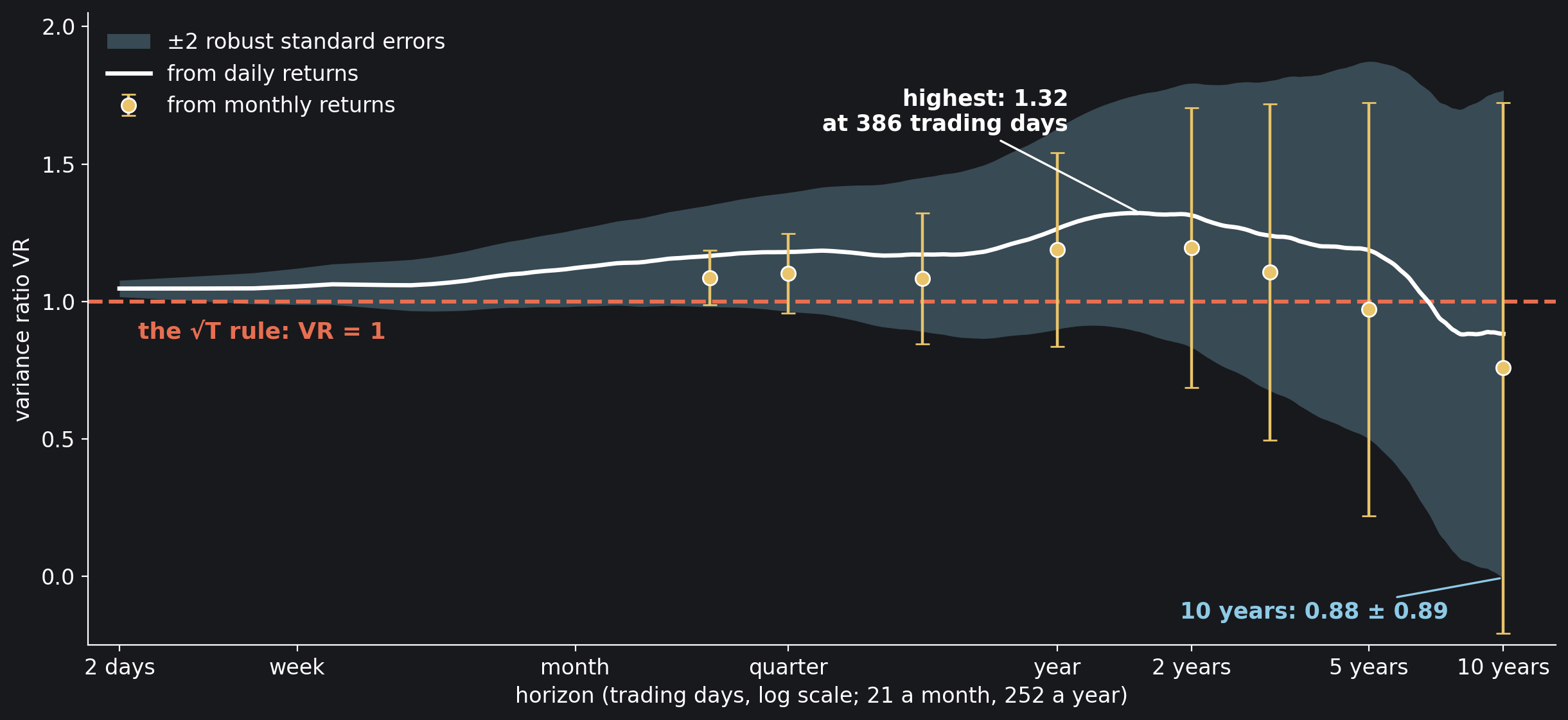
- Over 1926–2026 the square-root rule understated the market’s risk at every horizon from 2 trading days to 6.8 years: the variance ratio is 1.122 at a month, 1.264 at a year and highest, 1.322, near a year and a half.
- A century proves less than it seems: only the 2- and 3-day ratios lie more than two heteroskedasticity-robust standard errors from 1 (z* = 3.15 at 2 days), and at ten years the ratio of 0.882 has a robust standard error of 0.443: two of them either way span from about zero to about 1.8.
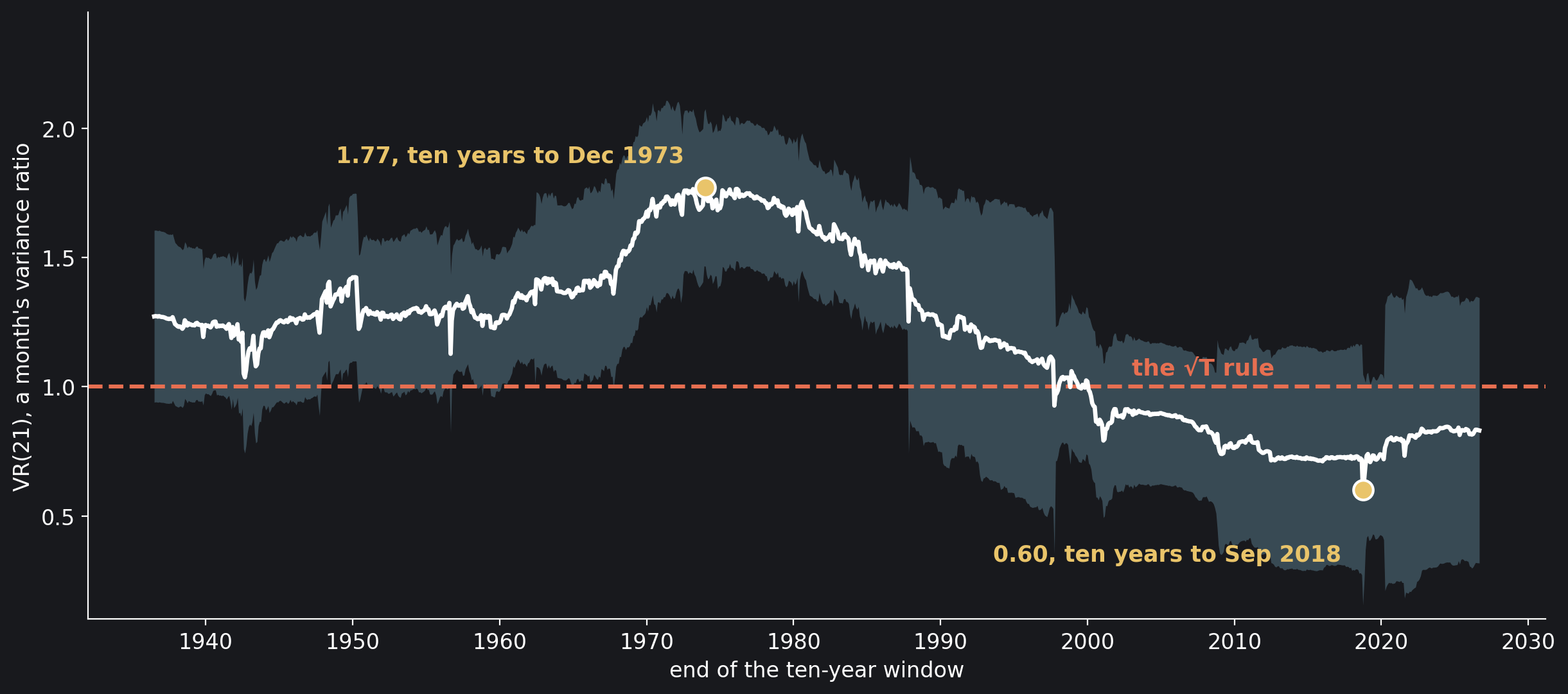
- The sign flipped around 2000. A week’s ratio was 1.152 over 1926–1999 (z* = 3.85) and 1.513 in the 1970s; over 2000–2026 it is 0.859 (z* = −2.37). A month’s ratio fell from 1.294 to 0.782, and is below 1 in every ten-year window ending after December 1999.
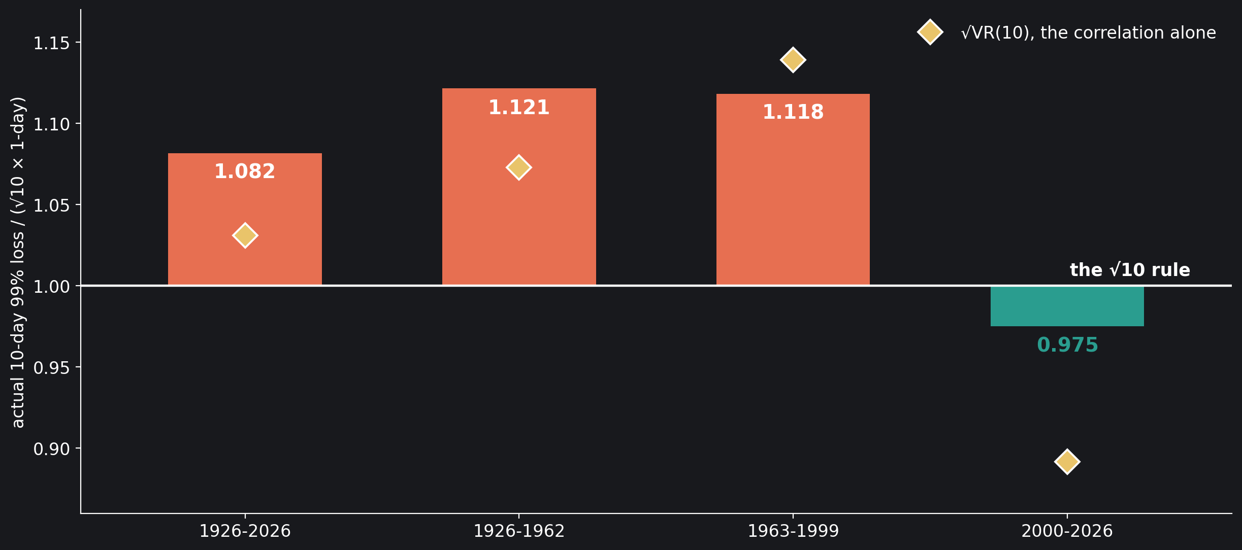
- Basel’s $\sqrt{10}$, measured on every overlapping ten-day window: the actual 99% ten-day loss was 1.082 times the rule’s over the century, 1.121 and 1.118 in 1926–1962 and 1963–1999, and 0.975 since 2000.
A Century of the Market
The data file holds one row per trading day: the return of French’s market portfolio, which his Data Library describes as the “value-weight return of all CRSP firms incorporated in the US and listed on the NYSE, AMEX, or NASDAQ” with good share and price data. CRSP’s returns include dividends. French publishes the market as an excess return over the one-month Treasury bill, so the file adds the bill back: total return = (Mkt-RF + RF) / 100. A second file holds the same for every month. The notebook works with log returns, $\ln(1 + R)$, because they add up: the return over $q$ days is the sum of the $q$ daily ones.
A Century of the Market
import numpy as np
import pandas as pd

day = pd.read_csv("data/french_market_daily.csv", index_col="date",
                  parse_dates=True)
mon = pd.read_csv("data/french_market_monthly.csv", index_col="month")
x = np.log1p(day["total_return"].to_numpy())    # daily log returns
xm = np.log1p(mon["total_return"].to_numpy())   # monthly log returns
yr = day.index.year.to_numpy()                  # each day's year
DAYS = 252                                      # trading days in a year
print(f"daily:   {len(x):,} trading days, {day.index[0]:%d %b %Y} to "
      f"{day.index[-1]:%d %b %Y}")
print(f"monthly: {len(xm):,} months, {mon.index[0]} to {mon.index[-1]}")

# daily:   26,317 trading days, 01 Jul 1926 to 31 Aug 2026
# monthly: 1,202 months, 1926-07 to 2026-08
Two series, 26,317 trading days and 1,202 months, both running from July 1926 to August 2026.
Before any test, the rule can be checked against the calendar. Multiply a day’s standard deviation by the square root of the number of trading days in a year and compare it with the standard deviation of the 99 whole calendar years from 1927 to 2025. One detail matters: the daily file has rows for Saturdays until 1952, so a year in the early decades held more than 252 trading days. The cell counts them and uses the file’s own average.
Root T Against the Calendar
sat = day.index.dayofweek == 5                  # rows that fall on a Saturday
cal = (yr >= 1927) & (yr <= 2025)               # whole calendar years only
years = pd.Series(x[cal], index=yr[cal]).groupby(level=0).agg(["sum", "size"])
per_year = years["size"].mean()                 # trading days in a year
sd = x[cal].std(ddof=1)                         # one day's spread
actual = years["sum"].std(ddof=1)               # the spread of the years
print(f"Saturday rows: {sat.sum():,}, the last on "
      f"{day.index[sat][-1]:%d %b %Y}")
print(f"trading days in a year, 1927-2025: {per_year:.1f}")
print(f"a day's spread x root {DAYS}:   {sd * np.sqrt(DAYS):.1%}")
print(f"a day's spread x root {per_year:.1f}: {sd * np.sqrt(per_year):.1%}")
print(f"{len(years)} calendar years: {actual:.1%}, "
      f"{actual / (sd * np.sqrt(per_year)):.3f} times the rule")

# Saturday rows: 1,158, the last on 24 May 1952
# trading days in a year, 1927-2025: 262.6
# a day's spread x root 252:   17.2%
# a day's spread x root 262.6: 17.5%
# 99 calendar years: 19.3%, 1.099 times the rule
The file has 1,158 Saturday rows, the last on 24 May 1952, and 262.6 trading days in an average year from 1927 to 2025. A day’s standard deviation times $\sqrt{262.6}$ says a year’s should be 17.5%; times the usual $\sqrt{252}$, 17.2%. The 99 calendar years actually spread by 19.3%, 1.099 times the rule. The square-root rule understated a year’s risk by about a tenth. The variance ratio says where the difference comes from, horizon by horizon.
The Variance Ratio
For a horizon of $q$ periods,
If returns are uncorrelated, the variance of the sum is the sum of the variances and $\mathrm{VR}(q) = 1$: the square-root rule. In general, Lo and MacKinlay showed, the excess over 1 is close to a weighted sum of the first $q-1$ autocorrelations $\rho(j)$, the weights falling in a straight line:
Days that follow through, positive autocorrelation, push the ratio above 1, and $q$ days then carry $\sqrt{\mathrm{VR}(q)\,q}$ days’ worth of risk instead of $\sqrt{q}$. Days that partly undo each other pull it below 1.
Their estimator (in their working paper of 1987, equations 10 to 18 and footnote 8) uses every overlapping $q$-period sum, not only the separate ones, and corrects both variances for bias. With $T$ returns and their mean $\hat\mu$,
If returns are uncorrelated with a constant variance, $\sqrt{T}\,(\widehat{\mathrm{VR}}(q) – 1)$ is approximately normal with variance $2(2q-1)(q-1)/(3q)$, which gives the statistic $z$. Market volatility is not constant, it comes in spells, so Lo and MacKinlay also gave a statistic $z^*$ that stays valid when the variance changes over time:
The cell writes the estimator down and prints three of the $\hat\delta(j)$, each of which would be close to 1 if the variance were constant.
The Variance Ratio
def deltas(x, qmax):                   # delta(j) for j = 1 .. qmax - 1
    e2 = (x - x.mean()) ** 2
    d = [(e2[j:] * e2[:-j]).sum() for j in range(1, qmax)]
    return len(x) * np.array(d) / e2.sum() ** 2

def vr(x, q, dl):                      # Lo and MacKinlay (1988)
    T, mu = len(x), x.mean()
    var1 = ((x - mu) ** 2).sum() / (T - 1)
    c = np.r_[0.0, np.cumsum(x)]       # every overlapping q-period sum
    m = q * (T - q + 1) * (1 - q / T)
    V = ((c[q:] - c[:-q] - q * mu) ** 2).sum() / m / var1
    j = np.arange(1, q)
    phi = 2 * (2 * q - 1) * (q - 1) / (3 * q)
    theta = ((2 * (q - j) / q) ** 2 * dl[:q - 1]).sum()
    se, se_r = np.sqrt(phi / T), np.sqrt(theta / T)
    return V, (V - 1) / se, (V - 1) / se_r, se, se_r

DL, DLm = deltas(x, 10 * DAYS), deltas(xm, 120)    # up to ten years
print(f"delta(1) {DL[0]:.2f}, delta(21) {DL[20]:.2f}, delta(252) {DL[251]:.2f}")

# delta(1) 5.90, delta(21) 2.74, delta(252) 1.61
They are far from 1: $\hat\delta(1) = 5.90$, $\hat\delta(21) = 2.74$ and $\hat\delta(252) = 1.61$. A day’s squared move and the squared move a day, a month or a year earlier tend to be large together: the market’s variance changes, in spells that last from days to years, and $z^*$ is the stricter test for it. At $q = 2$ the approximation above has a single term, $\mathrm{VR}(2) – 1 \approx \rho(1)$; the next cell checks it.
Two Days, One Correlation
e = x - x.mean()
rho1 = (e[1:] * e[:-1]).sum() / (e * e).sum()      # first autocorrelation
print(f"VR(2) = {vr(x, 2, DL)[0]:.4f}; 1 + rho(1) = {1 + rho1:.4f}")

# VR(2) = 1.0471; 1 + rho(1) = 1.0471
At two days the ratio is 1.0471 and $1 + \rho(1)$ is 1.0471: over the century, one day’s return and the next were positively correlated, and the variance ratio is that correlation in another form.
Over the Century
The cell computes the ratio at ten horizons from daily returns and at eight from monthly returns, with both statistics, both standard errors (se for $z$, se* for $z^*$) and $\sqrt{\mathrm{VR}}$, the factor by which the square-root rule is off. Horizons are counted in trading days: 21 is a month and 252 a year in today’s calendar; before 1952, with Saturday sessions, 252 trading days were about ten months.
Over the Century
H = {"2 days": 2, "week": 5, "2 weeks": 10, "month": 21, "quarter": 63,
     "half-year": 126, "year": 252, "2 years": 504, "5 years": 1260,
     "10 years": 2520}
M = {"2 months": 2, "quarter": 3, "half-year": 6, "year": 12,
     "2 years": 24, "3 years": 36, "5 years": 60, "10 years": 120}

def table(x, horizons, dl, unit):
    print(f"{unit:<10}{'q':>6}{'VR':>8}{'z':>8}{'z*':>8}{'se':>8}"
          f"{'se*':>8}{'root VR':>9}")
    for name, q in horizons.items():
        V, z, zr, se, se_r = vr(x, q, dl)
        print(f"{name:<10}{q:>6}{V:>8.3f}{z:>8.2f}{zr:>8.2f}{se:>8.3f}"
              f"{se_r:>8.3f}{np.sqrt(V):>9.3f}")

table(x, H, DL, "daily")
print()
table(xm, M, DLm, "monthly")

# daily          q      VR       z      z*      se     se*  root VR
# 2 days         2   1.047    7.65    3.15   0.006   0.015    1.023
# week           5   1.055    4.06    1.66   0.014   0.033    1.027
# 2 weeks       10   1.063    3.04    1.29   0.021   0.049    1.031
# month         21   1.122    3.88    1.75   0.031   0.070    1.059
# quarter       63   1.180    3.23    1.67   0.056   0.108    1.086
# half-year    126   1.171    2.15    1.22   0.079   0.140    1.082
# year         252   1.264    2.34    1.45   0.113   0.183    1.124
# 2 years      504   1.313    1.96    1.30   0.160   0.240    1.146
# 5 years     1260   1.186    0.74    0.54   0.253   0.343    1.089
# 10 years    2520   0.882   -0.33   -0.27   0.357   0.443    0.939
#
# monthly        q      VR       z      z*      se     se*  root VR
# 2 months       2   1.087    3.01    1.76   0.029   0.049    1.043
# quarter        3   1.102    2.38    1.41   0.043   0.073    1.050
# half-year      6   1.083    1.17    0.70   0.071   0.119    1.041
# year          12   1.188    1.74    1.07   0.108   0.176    1.090
# 2 years       24   1.196    1.24    0.77   0.158   0.254    1.094
# 3 years       36   1.107    0.55    0.35   0.196   0.306    1.052
# 5 years       60   0.971   -0.11   -0.08   0.255   0.375    0.985
# 10 years     120   0.759   -0.66   -0.50   0.363   0.483    0.871
From daily returns the ratio is above 1 at every horizon in the table up to two years: 1.047 at two days, 1.122 at a month, 1.264 at a year, 1.313 at two years. At 252 trading days $\sqrt{\mathrm{VR}}$ is 1.124: by this measure the rule misses a year’s risk by about 12%, close to the calendar years’ 1.099. Then the ratio turns down, to 1.186 at five years and 0.882 at ten. The monthly returns tell the same story at their own horizons: 1.188 at a year, 1.196 at two years, then 0.971 at five and 0.759 at ten. It is the shape James Poterba and Lawrence Summers described in 1988, returns “positively serially correlated over short horizons, and negatively autocorrelated over long horizons”, and that Eugene Fama and Kenneth French found the same year, with “large negative autocorrelations for return horizons beyond a year”.
The statistics are less sure than the shape. Against the constant-variance errors, $z$ is above 2 out to a year. Against the robust errors, wider at every horizon because volatility comes in spells, only the two-day ratio in the table passes: $z^* = 3.15$. At ten years one standard error is 0.357 under constant variance and 0.443 under the robust formula. A century holds ten separate ten-year spans, and ten draws cannot pin a ratio down. The next cell runs the daily ratio at every horizon from 2 trading days to 2,520 and finds where it peaks, where it crosses 1, and where its robust band clears 1.
Every Horizon
Q = np.arange(2, 10 * DAYS + 1)        # every horizon, 2 days to 10 years
R = np.array([vr(x, q, DL) for q in Q])
VR_d, SE_d = R[:, 0], R[:, 4]
top = Q[VR_d.argmax()]
under = Q[VR_d < 1][0]
print(f"highest VR: {VR_d.max():.3f} at {top} trading days "
      f"({top / DAYS:.1f} years)")
print(f"VR above 1 at every horizon up to {under - 1} trading days "
      f"({(under - 1) / DAYS:.1f} years)")
print(f"horizons with VR below 1: {np.sum(VR_d < 1)} of {len(Q)}, "
      f"all from {under} days on: {bool(np.all(VR_d[Q >= under] < 1))}")
print(f"robust bands clear of 1: {np.sum(np.abs(VR_d - 1) > 2 * SE_d)} "
      f"horizons, up to {Q[np.abs(VR_d - 1) > 2 * SE_d].max()} days")
print(f"at {Q[-1]} days: VR {VR_d[-1]:.3f} ± {2 * SE_d[-1]:.3f} "
      f"(two robust standard errors)")

# highest VR: 1.322 at 386 trading days (1.5 years)
# VR above 1 at every horizon up to 1709 trading days (6.8 years)
# horizons with VR below 1: 811 of 2519, all from 1710 days on: True
# robust bands clear of 1: 2 horizons, up to 3 days
# at 2520 days: VR 0.882 ± 0.887 (two robust standard errors)
The daily ratio peaks at 1.322 at 386 trading days, about a year and a half, stays above 1 at every horizon up to 1,709 trading days, 6.8 years, and is below 1 at every horizon from 1,710 on. Of the 2,519 horizons, only 2 and 3 days have a robust band that clears 1. Read the long end as a band, not a number: at ten years the estimate is 0.882 ± 0.887, two robust standard errors either way, a band from about zero to about 1.8. Figure 1 draws both.
The Sign Flipped
A century mixes several markets. The cell splits it into decades, with the first and last cut by the data (July 1926 to 1929, 2020 to August 2026), and for each prints the first-order autocorrelation $\rho(1)$, the variance ratio at 5 and at 21 trading days and the robust $z^*$ of each. The last two rows pool the years before and after 2000.
Decade by Decade
def ac1(x):                            # first-order autocorrelation
    e = x - x.mean()
    return (e[1:] * e[:-1]).sum() / (e * e).sum()

spans = [("1926-29", 1926, 1929)]
spans += [(f"{d}s", d, d + 9) for d in range(1930, 2020, 10)]
spans += [("2020-26", 2020, 2026), ("1926-1999", 1926, 1999),
          ("2000-2026", 2000, 2026)]
print(f"{'':<11}{'days':>7}{'rho(1)':>8}{'VR(5)':>8}{'z*':>7}"
      f"{'VR(21)':>8}{'z*':>7}")
for name, lo, hi in spans:
    g = x[(yr >= lo) & (yr <= hi)]
    dl = deltas(g, 21)
    v5, v21 = vr(g, 5, dl), vr(g, 21, dl)
    print(("\n" if name == "1926-1999" else "")
          + f"{name:<11}{len(g):>7,}{ac1(g):>+8.3f}{v5[0]:>8.3f}"
          f"{v5[2]:>7.2f}{v21[0]:>8.3f}{v21[2]:>7.2f}")

#               days  rho(1)   VR(5)     z*  VR(21)     z*
# 1926-29      1,037  +0.133   0.961  -0.13   1.260   0.45
# 1930s        2,988  +0.052   1.094   1.57   1.240   1.82
# 1940s        2,918  +0.157   1.204   2.64   1.424   2.61
# 1950s        2,598  +0.127   1.100   1.60   1.250   1.88
# 1960s        2,489  +0.202   1.374   3.83   1.678   3.68
# 1970s        2,526  +0.289   1.513   8.42   1.686   4.98
# 1980s        2,528  +0.131   1.160   1.29   1.239   0.97
# 1990s        2,528  +0.078   1.102   1.53   1.020   0.14
# 2000s        2,515  -0.062   0.837  -2.08   0.763  -1.26
# 2010s        2,516  -0.038   0.921  -1.09   0.737  -1.68
# 2020-26      1,674  -0.151   0.848  -1.02   0.846  -0.51
#
# 1926-1999   19,612  +0.111   1.152   3.85   1.294   3.58
# 2000-2026    6,705  -0.081   0.859  -2.37   0.782  -1.67
Every decade from the 1920s to the 1990s had positive day-to-day autocorrelation, and every one but the first had a weekly ratio above 1. The 1960s and 1970s stand out: $\rho(1)$ of +0.202 and +0.289, weekly ratios of 1.374 and 1.513, monthly ratios of 1.678 and 1.686, with $z^*$ between 3.68 and 8.42. The 1940s also clear two robust standard errors, at 2.64 and 2.61; the other decades before 2000 point the same way without clearing them, except the weekly ratio of 1926–29, 0.961. Since 2000 every decade’s autocorrelation is negative, from −0.038 to −0.151, and every ratio is below 1: weekly 0.837, 0.921 and 0.848, monthly 0.763, 0.737 and 0.846. Decade by decade only the 2000s’ weekly ratio clears two robust standard errors ($z^* = -2.08$). Pooled, the difference is plain: before 2000 the weekly ratio was 1.152 ($z^* = 3.85$) and the monthly 1.294 (3.58); since, 0.859 ($-2.37$) and 0.782 ($-1.67$). Before 2000 the square-root rule understated a week’s and a month’s risk; since 2000 it has overstated them, measurably for the week.
Why the old index returns followed through is not settled here. One candidate is mechanical: the stocks in an index do not all trade at the close, so a stale price catches up the next day and the index looks correlated even when no stock is. Lo and MacKinlay modelled exactly this in 1990 and found it too small for what they had measured: the largest autocorrelation it implied for a weekly equal-weighted index was 7.5 percent, against the 30 percent they had reported, and in the working-paper version they concluded that the evidence gave “little support for nonsynchronous-trading as an important source of spurious correlation in the returns of common stock.” Their index was weekly and equal-weighted, not this daily value-weighted one, so the notebook leaves the cause open.
The next cell follows the monthly ratio through time, over the ten calendar years ending each month, with its robust band, and counts the windows whose band lies wholly above or wholly below 1.
Ten Years at a Time
ends = day.groupby(day.index.to_period("M")).tail(1).index   # month ends
ends = ends[ends >= day.index[0] + pd.DateOffset(years=10, days=-1)]
roll = []
for end in ends:                       # the ten calendar years to each end
    g = x[(day.index > end - pd.DateOffset(years=10)) & (day.index <= end)]
    V, z, zr, se, se_r = vr(g, 21, deltas(g, 21))
    roll.append((end, V, se_r))
roll = pd.DataFrame(roll, columns=["end", "VR", "se"]).set_index("end")
up = roll["VR"] - 2 * roll["se"] > 1   # band wholly above 1
down = roll["VR"] + 2 * roll["se"] < 1  # band wholly below 1
since = roll.index[roll["VR"] >= 1][-1]
print(f"{len(roll):,} windows, ending {roll.index[0]:%b %Y} to "
      f"{roll.index[-1]:%b %Y}")
print(f"highest VR(21) {roll['VR'].max():.3f}, ending "
      f"{roll['VR'].idxmax():%b %Y}; lowest {roll['VR'].min():.3f}, "
      f"ending {roll['VR'].idxmin():%b %Y}")
print(f"band above 1: {up.sum()} windows, the last ending "
      f"{roll.index[up][-1]:%b %Y}; band below 1: {down.sum()}")
print(f"VR(21) below 1 in every window ending after {since:%b %Y}")

# 1,083 windows, ending Jun 1936 to Aug 2026
# highest VR(21) 1.771, ending Dec 1973; lowest 0.601, ending Sep 2018
# band above 1: 398 windows, the last ending Sep 1987; band below 1: 0
# VR(21) below 1 in every window ending after Dec 1999
Over 1,083 windows the monthly ratio ran from 1.771, in the ten years to December 1973, down to 0.601, in the ten years to September 2018. In 398 windows its band lay wholly above 1, the last of them ending in September 1987; in none did it lie wholly below. The ratio is below 1 in every window ending after December 1999. Figure 2 shows the turn.
Basel’s Square Root of Ten
The 1996 amendment states its standard in two lines: “In calculating the value-at-risk, a 99th percentile, one-tailed confidence interval is to be used”, and “the minimum ‘holding period’ will be ten trading days.” The cell measures the shortcut in those terms. The one-day loss is the 1% quantile of the daily log returns, sign reversed; the rule multiplies it by $\sqrt{10}$; the actual ten-day loss is the 1% quantile of every overlapping ten-day log return. It does this over the century and in three spans of about 37, 37 and 27 years, and prints beside each $\sqrt{\mathrm{VR}(10)}$, the ratio the correlation alone would give if the shape of the tails stayed the same. A last line repeats the century at the 99.9th percentile.
Basel’s Square Root of Ten
def losses(g, p):                      # the loss at probability p
    c = np.r_[0.0, np.cumsum(g)]
    ten = c[10:] - c[:-10]             # every overlapping 10-day return
    one = -np.quantile(g, p)
    return one, np.sqrt(10) * one, -np.quantile(ten, p)

SPANS = {"1926-2026": (1926, 2026), "1926-1962": (1926, 1962),
         "1963-1999": (1963, 1999), "2000-2026": (2000, 2026)}
print(f"{'99%':<11}{'1 day':>8}{'x root 10':>11}{'10 days':>9}"
      f"{'actual/rule':>13}{'root VR(10)':>13}")
basel = {}
for name, (lo, hi) in SPANS.items():
    g = x[(yr >= lo) & (yr <= hi)]
    one, rule10, ten = losses(g, 0.01)
    basel[name] = (ten / rule10, np.sqrt(vr(g, 10, deltas(g, 10))[0]))
    print(f"{name:<11}{one:>8.2%}{rule10:>11.2%}{ten:>9.2%}"
          f"{basel[name][0]:>13.3f}{basel[name][1]:>13.3f}")
_, rule10, ten = losses(x, 0.001)
print(f"\n99.9%, 1926-2026: {ten:.2%} against {rule10:.2%}, {ten / rule10:.3f}")

# 99%           1 day  x root 10  10 days  actual/rule  root VR(10)
# 1926-2026     3.12%      9.86%   10.66%        1.082        1.031
# 1926-1962     3.55%     11.24%   12.60%        1.121        1.073
# 1963-1999     2.16%      6.84%    7.65%        1.118        1.139
# 2000-2026     3.46%     10.94%   10.67%        0.975        0.892
#
# 99.9%, 1926-2026: 22.75% against 21.57%, 1.055
Over the century the market’s one-day loss at 99% was 3.12%; $\sqrt{10}$ times it is 9.86%, while the actual ten-day loss was 10.66%, 1.082 times the rule’s number. At 99.9% the actual was 22.75% against the rule’s 21.57%, 1.055 times. The actual ten-day loss exceeded the rule’s number by 12.1% in 1926–1962 and by 11.8% in 1963–1999. Since 2000 it has run the other way: a ten-day loss of 10.67% against the rule’s 10.94%, a ratio of 0.975. The correlation points the same way in every span, $\sqrt{\mathrm{VR}(10)}$ of 1.031, 1.073, 1.139 and 0.892, but it does not set the size: in the far tail the ten-day returns have a shape of their own. Figure 3 sets the four side by side.
What the Numbers Show
The square-root rule assumes that one day’s return says nothing about the next, and the US market has not obliged for long in either direction. Before 2000 it followed through: a day’s risk scaled by $\sqrt{T}$ fell short of a week’s and a month’s, and the actual ten-day loss at 99% was about 12% larger than Basel’s $\sqrt{10}$ gave, in each half of 1926–1999. Since 2000 the days partly undo each other: the weekly and monthly ratios are below 1, and the market’s ten-day loss at 99% came in 2.5% below the $\sqrt{10}$ rule’s. Over the whole century the two eras average out to a rule that understated risk out to 6.8 years, but only the shortest horizons are measured precisely. At ten years a century of data cannot tell mean reversion from the square-root rule.
The variance ratio tests only one of the rule’s assumptions. Francis Diebold, Andrew Hickman, Atsushi Inoue and Til Schuermann showed in 1997 that converting a one-day volatility estimate to $h$ days by scaling by $\sqrt{h}$ “produces overestimates of the variability of long-horizon volatility”. Jón Daníelsson and Jean-Pierre Zigrand showed in 2006 that when returns can jump, the rule understates the quantile, the more so the longer the horizon, the more frequent the jumps and the higher the confidence level.
The one action the numbers support is a measurement. Before multiplying a daily number by $\sqrt{T}$, compute the variance ratio at that horizon over the years being used: $\sqrt{\mathrm{VR}}$ is the factor by which the rule is off. Over the century it is 1.124 for a year. For a month the ratio was 1.294 before 2000 and is 0.782 since: the same multiplication was too small then and is too large now. These are one market’s hundred years, and none of it is a forecast.
Sources
- A. W. Lo and A. C. MacKinlay, “Stock Market Prices Do Not Follow Random Walks: Evidence from a Simple Specification Test”, The Review of Financial Studies 1 (1988) 41–66, doi:10.1093/rfs/1.1.41. The estimator and its two statistics are read in the working paper, NBER Working Paper 2168 (February 1987).
- A. W. Lo and A. C. MacKinlay, “An econometric analysis of nonsynchronous trading”, Journal of Econometrics 45 (1990) 181–211, doi:10.1016/0304-4076(90)90098-E. The 7.5 and 30 percent and the quoted conclusion are read in the working paper, NBER Working Paper 2960 (May 1989).
- J. M. Poterba and L. H. Summers, “Mean reversion in stock prices: Evidence and Implications”, Journal of Financial Economics 22 (1988) 27–59, doi:10.1016/0304-405X(88)90021-9; the quoted words are from the abstract of the working paper, NBER Working Paper 2343 (1987).
- E. F. Fama and K. R. French, “Permanent and Temporary Components of Stock Prices”, Journal of Political Economy 96 (1988) 246–273, doi:10.1086/261535.
- Basle Committee on Banking Supervision, Amendment to the Capital Accord to incorporate market risks, January 1996: Part B, section B.4, Quantitative standards, (b) and (c).
- F. X. Diebold, A. Hickman, A. Inoue and T. Schuermann, “Converting 1-Day Volatility to h-Day Volatility: Scaling by √h is Worse than You Think”, Wharton Financial Institutions Center Working Paper 97-34 (1997), RePEc; condensed as “Scale Models”, Risk 11 (1998) 104–107.
- J. Daníelsson and J.-P. Zigrand, “On time-scaling of risk and the square-root-of-time rule”, Journal of Banking & Finance 30 (2006) 2701–2713, doi:10.1016/j.jbankfin.2005.10.002.
- K. R. French, Data Library: the Fama/French 3 Factors, daily and monthly, built from the CRSP database of August 2026.
Every number in this notebook is computed by its own cells from the two data files.
Working on a pricing model or risk system? Let’s talk.
Also on
 YouTubeDoes Risk Grow With the Square Root of Time? The Variance Ratio on US Stocks Since 1926This notebook in plain words, in a few minutes.Watch on YouTube →FacebookThe walkthrough on our Facebook PageThe short film, with its comments.Discuss on Facebook →The same notebook on KaggleRun it in the browser, cell by cell, on Kaggle.Run the notebook →