A Coin With No Memory Still Looks Cold

A Result That Stood for Thirty Years

In 1985 Gilovich, Vallone and Tversky asked whether basketball players get hot. They took shooting records, looked at what happened immediately after a make, and compared it with what happened immediately after a miss. The two numbers were about the same. The hot hand, they concluded, is something spectators see in randomness rather than something shooters do.

The finding became a fixture. It is the standard example of humans inventing pattern in noise, and it has been repeated in psychology courses, popular books and trading floors for three decades.

In 2018 Miller and Sanjurjo pointed out that the measurement itself is biased. Not the data, not the sport, not the players. The procedure of looking at the flips that follow a head is biased downward, and in short sequences the bias is enormous.

The same argument in two minutes. The written version, with the code, is below.

The Bias, in Four Flips

Here is the whole thing, with no basketball in it at all.

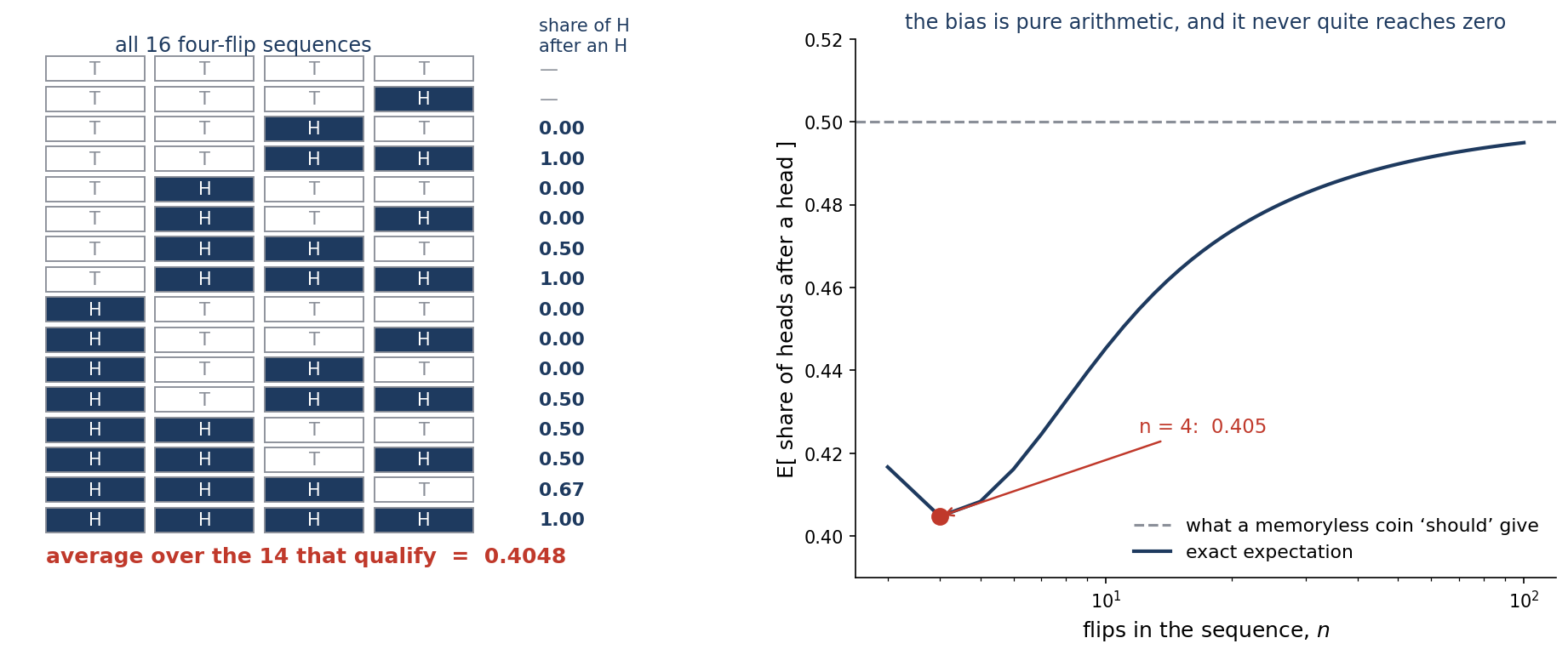
Flip a fair coin four times. Write down the sequence. Now find every flip that came immediately after a head, and ask what fraction of those were heads. If the sequence is HHTH, the flips after a head are the second (H) and the fourth (H), giving a share of 1.00. If it is HTHT, they are the second (T) and the fourth (T), giving 0.00.

Do this for all sixteen possible sequences. Two of them, TTTT and TTTH, have no head before the last position and are discarded because the question cannot be asked. Average the remaining fourteen.

The answer is 0.4048, not 0.5.

Nothing about the coin has changed. Each flip is still independent, still fair, and the conditional probability that any particular flip is a head given the one before it was a head is exactly one half. The number came out low because of how the flips were selected.

The intuition, once seen, is hard to unsee. Asking for a flip that follows a head uses up a head to qualify it. In a finite sequence, heads are a finite resource, so the flips that survive the filter are drawn from a pool that is very slightly depleted of them. It is sampling without replacement wearing a disguise.

Why a Ratio Is Not a Ratio of Averages

Write $X_1, \ldots, X_n$ for the flips, and count

The estimator everybody uses is the share $\hat{p} = B/A$. Its numerator and denominator are both perfectly well behaved: $\mathbb{E}[B] = (n-1)/4$ and $\mathbb{E}[A] = (n-1)/2$, so

But that is not the quantity being reported. What gets reported is $\mathbb{E}[B/A]$, and the expectation of a ratio is not the ratio of expectations. $A$ and $B/A$ are negatively related: the sequences with many heads, which get a large denominator, are also the sequences where the share is pulled toward one half, while the sequences with a single head give a share of either 0.00 or 1.00 on the strength of one flip. Averaging those extremes with equal weight, rather than weighting by how much evidence each sequence carries, is what drags the mean below one half.

This is not a subtlety that vanishes with care. It is arithmetic, and it is present in every sequence of every length.

Measuring It Exactly

Enumeration settles $n = 4$ by hand, but sixteen sequences become a million by $n = 20$ and the question is how the bias behaves as the record gets longer. A short dynamic program over the state $(\text{last flip}, A, B)$ gives the exact expectation for any $n$ without enumerating anything, and the brute force is kept alongside it as a check.

import itertools
import numpy as np
import matplotlib
matplotlib.use("Agg")
import matplotlib.pyplot as plt
from collections import defaultdict

NAVY, TEAL, GREY, RED = "#1e3a5f", "#2a9d8f", "#8a8f98", "#c0392b"

def exact_expectation(n):
    """E[ share of heads on the flip AFTER a head ] over n fair flips.

    Exact, by dynamic programming over (last flip, A, B) rather than by
    enumerating 2**n sequences."""
    cur = {(1, 0, 0): 1, (0, 0, 0): 1}
    for _ in range(n - 1):
        nxt = defaultdict(int)
        for (last, a, b), c in cur.items():
            for new in (0, 1):
                nxt[(new, a + last, b + (last & new))] += c
        cur = nxt
    tot = num = 0
    for (_, a, b), c in cur.items():
        if a:
            num += c * (b / a)
            tot += c
    return num / tot

# the DP must agree with straight enumeration wherever enumeration is feasible
for n in (3, 4, 5, 6, 10):
    vals = []
    for s in itertools.product([0, 1], repeat=n):
        after = [s[i + 1] for i in range(n - 1) if s[i] == 1]
        if after:
            vals.append(np.mean(after))
    assert abs(np.mean(vals) - exact_expectation(n)) < 1e-12, n

ns = list(range(3, 101))
E = [exact_expectation(n) for n in ns]

fig, (axL, axR) = plt.subplots(1, 2, figsize=(12.5, 5.4), facecolor="white",
                               gridspec_kw={"width_ratios": [1.05, 1.0]})

# left: every four-flip sequence and the share it reports
seqs = list(itertools.product([0, 1], repeat=4))
rows, vals = [], []
for s in seqs:
    after = [s[i + 1] for i in range(3) if s[i] == 1]
    rows.append(s)
    vals.append(np.mean(after) if after else None)
y = len(rows)
for s, v in zip(rows, vals):
    y -= 1
    for j, f in enumerate(s):
        axL.add_patch(plt.Rectangle((j, y), .9, .82,
                      facecolor=(NAVY if f else "white"), edgecolor=GREY, lw=.9))
        axL.text(j + .45, y + .41, "H" if f else "T", ha="center", va="center",
                 fontsize=10, color=("white" if f else GREY))
    axL.text(4.5, y + .41, "—" if v is None else f"{v:.2f}", ha="left", va="center",
             fontsize=10.5, color=(GREY if v is None else NAVY),
             fontweight=("normal" if v is None else "bold"))
axL.set_xlim(-.3, 6.4)
axL.set_ylim(-1.5, 16.4)
axL.axis("off")
axL.text(1.8, 16.0, "all 16 four-flip sequences", ha="center", fontsize=11.5, color=NAVY)
axL.text(4.5, 16.0, "share of H\nafter an H", ha="left", fontsize=10, color=NAVY)
good = [v for v in vals if v is not None]
axL.text(0, -1.0, f"average over the 14 that qualify  =  {np.mean(good):.4f}",
         fontsize=12, color=RED, fontweight="bold")

# right: the exact expectation against sequence length
axR.axhline(.5, color=GREY, ls="--", lw=1.5,
            label="what a memoryless coin ‘should’ give")
axR.plot(ns, E, "-", color=NAVY, lw=2.0, label="exact expectation")
axR.plot([4], [exact_expectation(4)], "o", color=RED, ms=9, zorder=5)
axR.annotate(f"n = 4:  {exact_expectation(4):.3f}", xy=(4, exact_expectation(4)),
             xytext=(12, .425), fontsize=11, color=RED,
             arrowprops=dict(arrowstyle="->", color=RED, lw=1.2))
axR.set_xscale("log")
axR.set_xlabel("flips in the sequence, $n$", fontsize=12)
axR.set_ylabel("E[ share of heads after a head ]", fontsize=12)
axR.set_ylim(.39, .52)
axR.legend(fontsize=10.5, frameon=False, loc="lower right")
axR.spines["top"].set_visible(False)
axR.spines["right"].set_visible(False)
axR.set_title("the bias is pure arithmetic, and it never quite reaches zero",
              fontsize=11.5, color=NAVY)

plt.tight_layout(pad=1.5)
fig.savefig("fig_1.png", dpi=150, bbox_inches="tight")

What the Picture Says

The left panel is the argument in full. Every row is a sequence you could write down yourself, every share is one division, and the average of the fourteen answerable rows is visibly below one half. There is no modelling and no estimation to disagree with.

The right panel says how long the problem lasts. The bias is deepest at $n = 4$, where it is $-0.095$. It is still $-0.055$ at ten flips and $-0.026$ at twenty. By a hundred flips it has shrunk to $-0.005$, which is when it stops mattering for most purposes. The curve approaches one half but never touches it, because the selection effect is present at every finite length.

The uncomfortable part is where that range sits. Controlled shooting experiments, the ones that measure a player taking a fixed set of attempts under identical conditions, live at exactly the sequence lengths where the bias is largest. The original analysis compared the after-a-make share against a benchmark of one half. The correct benchmark was several points lower, which means a player shooting genuinely better after a make could still produce a number that looked like no effect at all.

What This Does and Does Not Prove

It does not prove the hot hand exists. That is a claim about basketball, and this post contains no basketball.

What it proves is narrower and more useful: the standard test was biased against finding the effect it was looking for. When Miller and Sanjurjo applied the correction to the original controlled-shooting data, the conclusion moved the other way. A result that had been treated as settled for thirty years turned out to rest on an estimator nobody had checked.

The transferable lesson has nothing to do with sport. Look at what happened after X is not a description of the data. It is a conditioning rule, and conditioning rules have their own arithmetic that runs whether or not you have thought about it. Any time a study selects observations by a property of the observation before them, the same depletion applies. Streaks in anything, runs of good weeks, what happened the day after a big move: all of them are the same shape, and all of them need a benchmark computed under the null rather than assumed from first principles.

The cheapest protection is the one used above. Simulate the null with the exact selection rule you actually applied, and see what number it gives you before you decide whether the real number is surprising.

Interested in applying these ideas to your work? Get in touch.