
The Earthquake That Changes the Clock
The second shock
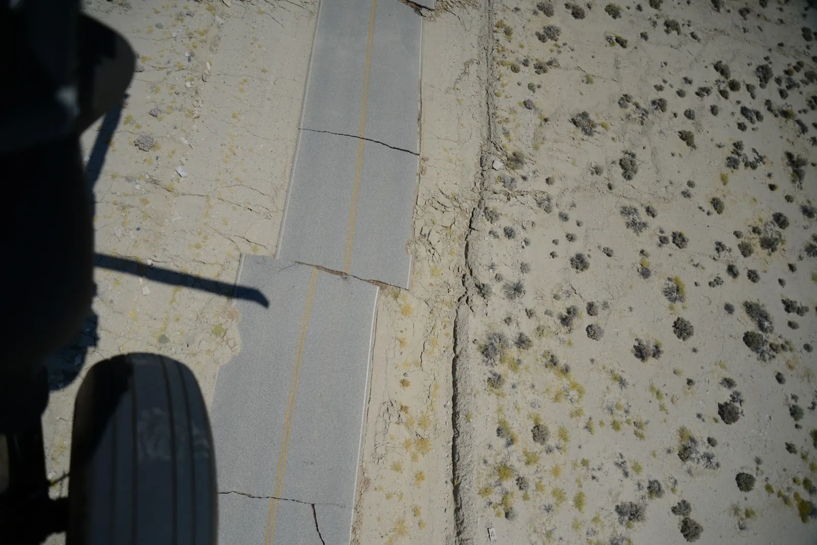
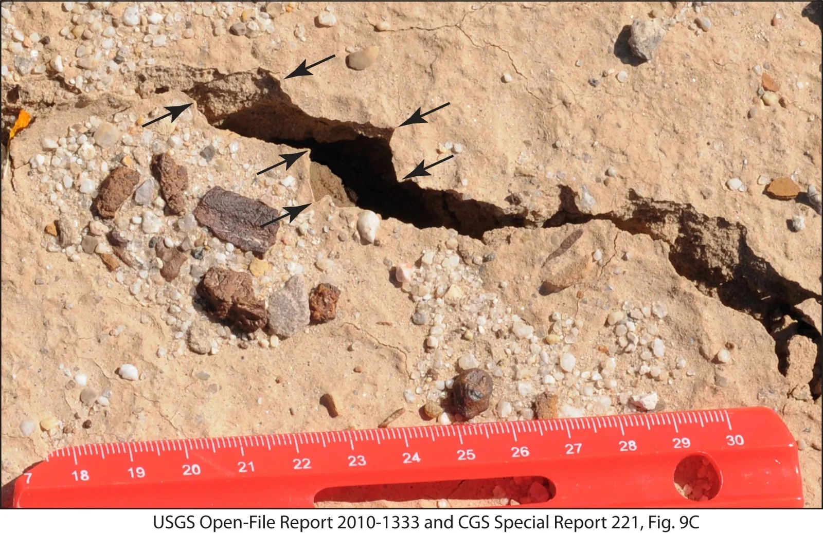
On July 4, 2019, a magnitude 6.4 earthquake struck near Ridgecrest. The next day, a magnitude 7.1 earthquake followed. What had looked like the main event became part of a larger sequence. [1]
A clock that assigns the same earthquake rate to every day cannot respond to that first shock. A clock with memory can. Each observed earthquake raises its rate; quiet time lets the rate fall again.
We tested those two ideas on a fixed study box covering Southern California and northern Baja California. We fitted the clocks using 2000–2014, froze their parameters, and scored them on 2015–2025. The simple exponential-memory clock gained 2.31 nats per earthquake over the constant clock at the lowest cutoff. Memory won at every magnitude cutoff tested, including when we left 2019 out of the scoring.
The richer Omori model also improved the score, but pressed against a parameter limit. We treat its results as indicative.
One average hides the sequence
Our public USGS catalog extract covers 32–37 degrees north and 122–114 degrees west. The rectangle reaches into northern Baja California, Mexico. We count cataloged earthquakes of magnitude 3.5 and above. [2]
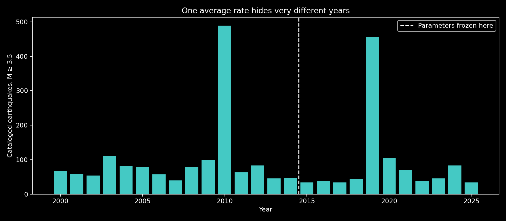
There are 1,452 events in the fifteen training years and 984 in the eleven test years. The training average is about one event every 3.8 days. A constant-rate clock takes that average into every subsequent day, whether the ground has been quiet or a large earthquake has just occurred.
The largest training year is 2010, with 489 events. It includes the magnitude 7.2 El Mayor–Cucapah earthquake in Baja California; 393 of that year’s events lie south of 32.7°N. The spike belongs to a cross-border catalog, not just California.
The test-year counts make that simplification visible. There were 44 qualifying events in 2018, 456 in 2019, and 106 in 2020.
The average alone does not say when events gather together. That is the question we ask the second clock to answer.
A clock that remembers
For a Poisson clock, the conditional rate is a constant, $\lambda(t)=r$. The chance of another event in a very short interval of length $\Delta t$ is approximately $r\Delta t$, whatever has just happened.
The simplest memory clock replaces that constant by
$$\lambda(t)=\mu+\sum_{t_i\lt t}\frac{n}{\tau}\exp\left(-\frac{t-t_i}{\tau}\right).$$
Here $\mu$ is the background rate. Each earlier event adds a pulse, and each pulse decays on a timescale $\tau$. The fitted exponential clock has a decay timescale of about 3.2 hours at the lowest magnitude cutoff.
Our second memory clock allows larger events to contribute larger pulses and replaces exponential decay by a slower Omori-shaped tail:
$$\lambda(t)=\mu+n\sum_{t_i\lt t}w_i\frac{p-1}{c}\left(1+\frac{t-t_i}{c}\right)^{-p},\qquad w_i=\frac{\exp\{\alpha(M_i-M_0)\}}{\overline{\exp\{\alpha(M-M_0)\}}_{\mathrm{train}}}.$$
The denominator is fixed from training magnitudes. The temporal kernel integrates to one for $p>1$; the magnitude weight controls the size of each contribution. This is a simplified temporal ETAS-style model, following an established statistical approach to earthquake sequences. It has no spatial triggering model. [3]
USGS also uses statistical models of aftershock activity, including models with Omori decay. Our small comparison is not a replacement for their operational forecasts. [4]
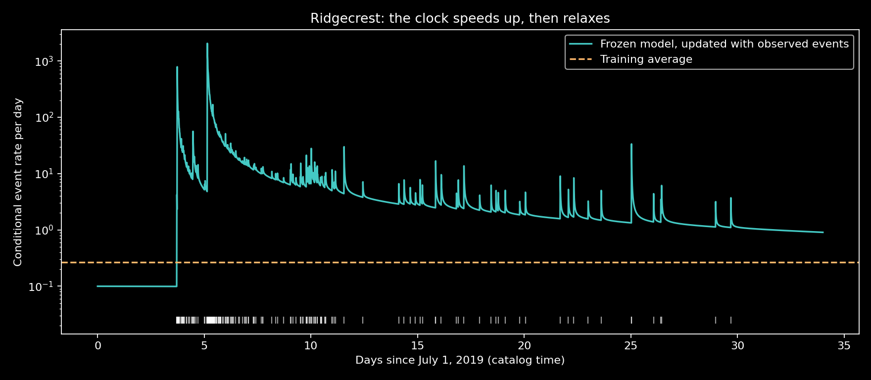
The first large shock raises the clock. The next one raises it again. The model responds to events after they arrive; this picture does not show it predicting either large shock in advance.
Make the clock answer for unseen years
We score a clock by adding the log rate it assigned immediately before each observed event, then subtracting its integrated rate over the entire test period:
$$L=\sum_{i\in\mathrm{test}}\log\lambda(t_i)-\int_{\mathrm{test}}\lambda(t)\,dt.$$
The first term rewards putting rate where events occur. The second charges for assigning rate everywhere else. Keeping the rate high all the time is therefore expensive.
At magnitude 3.5 and above, the exponential clock gains 2.31 nats per event over the constant clock. In plain words, exponentiating that average log-score gain gives exp(2.31) ≈ 10: a likelihood advantage of about tenfold per earthquake for its account of the test years, including the quiet intervals. This is not a tenfold probability of predicting the next shock.
The Omori-and-magnitude clock gains 2.84 nats per event. Its bound-sensitive fit makes that comparison indicative; the exponential result is the firmer finding.
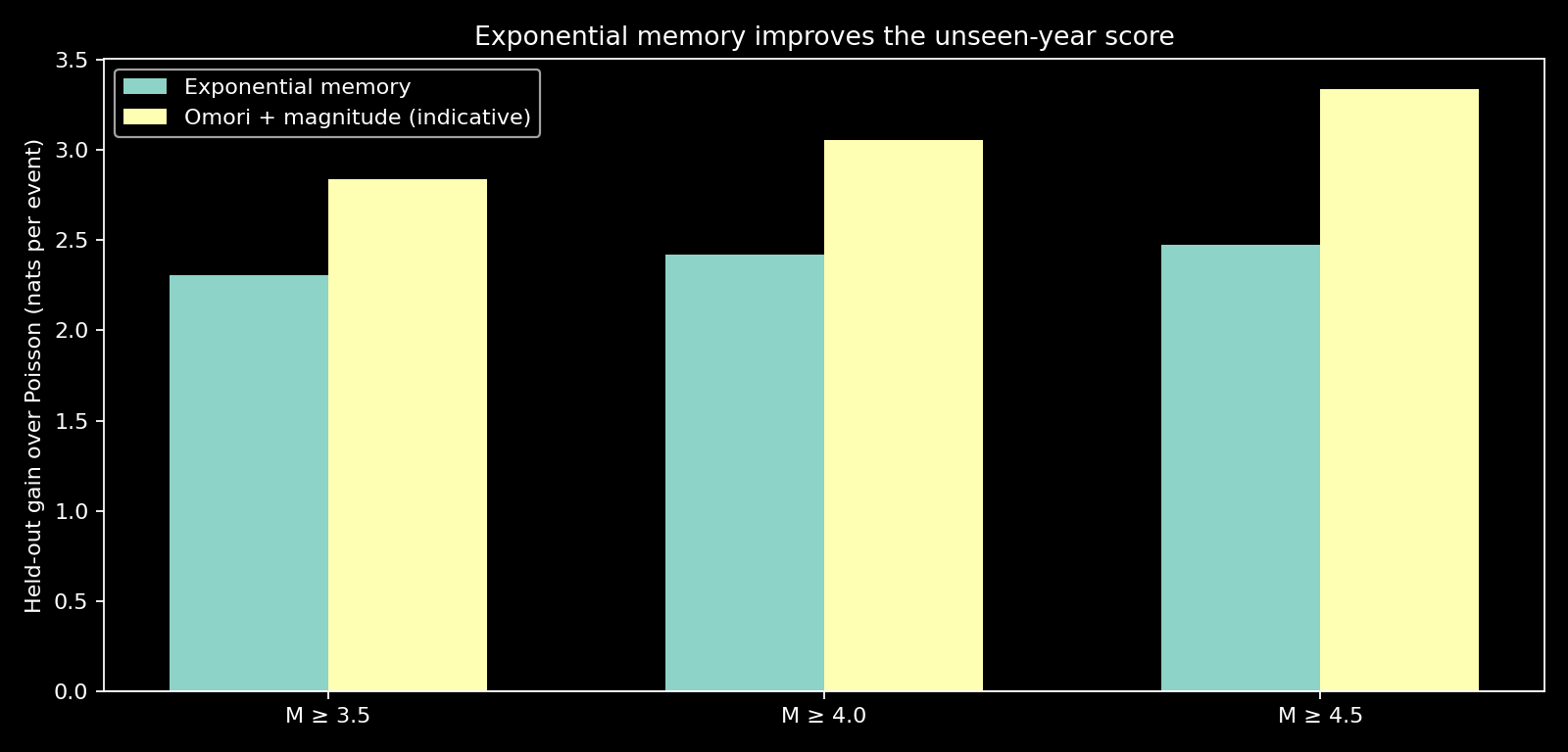
Ridgecrest is a major contributor: 2019 supplies 456 of the 984 test events. Remove that entire year from scoring, while preserving the actual event history available to later dates, and the gains remain positive: 0.71 nats per event for exponential memory and 1.00 for Omori-and-magnitude memory.
The conclusion is therefore broader than one exceptional year. Even the simpler exponential clock captures useful timing structure outside 2019.
Algorithm — Compare a constant clock with a clock that remembers
1. Fix the geographic box, magnitude cutoffs and training/test dates.
2. Download and preserve the catalog, keeping two earlier years as initial history.
3. Estimate each clock on training observations only.
4. Freeze its parameters; update its history as test events arrive.
5. Score event timing and the rate assigned between events.
6. Repeat at the higher cutoffs and report the result with 2019 excluded from scoring.
What a winning clock still gets wrong
The Omori model reaches the imposed 0.979 upper limit on its branching coefficient at all three cutoffs. Its slow tail leaves roughly 31% of each event’s kernel beyond fifteen years, longer than the training window. The gains partly reflect this bound-sensitive fit; 0.979 is not a measured fraction of physically triggered earthquakes. Magnitude weighting and the Omori tail enter together, so their separate benefits are unresolved.
These are revised catalog records, and small events can be missed after large shocks. Higher cutoffs check sensitivity, not completeness. [4] The model omits spatial triggering and influences outside the box; parameter uncertainty is not quantified. Its rate updates after observed events, so neither the Ridgecrest picture nor a close total count establishes an advance forecast.
The defensible result is narrower, and more useful, than a prophecy: an average event rate throws away information that the recent sequence contains. In this fixed study, a clock allowed to remember that sequence described unseen event times better.
Sources
- U.S. Geological Survey, “Five Years After the Ridgecrest Earthquake Sequence” (2024). Supports the opening sequence and magnitudes.
- U.S. Geological Survey, “Earthquake Catalog API Documentation” and “ANSS Comprehensive Earthquake Catalog (ComCat) Documentation”. Public event records; the exact query and downloaded bytes are archived with this study.
- Y. Ogata, “Statistical Models for Earthquake Occurrences and Residual Analysis for Point Processes,” Journal of the American Statistical Association 83, no. 401 (1988), 9–27. Listed in the author’s publication record.
- U.S. Geological Survey, “Aftershock Forecast Scientific Background” and “Aftershock Forecast Overview”. Statistical aftershock models, magnitude dependence, decay and early catalog incompleteness.
The event counts, fitted clocks, scores and figures are computed by the archived scripts from the preserved public catalog. Fits are saved once and reused. The kernel integrals and all six held-out likelihoods were checked independently.
Interested in applying these ideas to your work? Get in touch.