
In May 2019 The Hamilton Project published Recession Ready, a book of proposals for fighting the next recession before Congress had time to argue about it. Its third chapter was by Claudia Sahm, then an economist at the Board of Governors of the Federal Reserve System, and it proposed sending money: lump-sum payments to every adult, paid out automatically early in a recession. Automatic money needs a trigger anyone can check, and she wrote it in one sentence. The payments “would be made to individuals when the three-month average national unemployment rate rises by at least 0.50 percentage points relative to its low in the previous 12 months.”
She tried it on the unemployment rates known at each moment since 1970 and found that “Even a modest rise in the unemployment rate such as 0.50 percentage points … has occurred only during or closely following recessions. In other words, by this rule the stimulus payments would have been triggered only in recessions.” The trigger now has a name of its own. FRED, the database of the Federal Reserve Bank of St. Louis, publishes it every month as the Sahm Rule Recession Indicator.
By the summer of 2024 it stood at 0.43, and its author was the first to doubt it. “A recession is not imminent, even though the Sahm rule is close to triggering,” Sahm, by then chief economist at New Century Advisors, wrote on 26 July in her newsletter Stay-At-Home Macro. “The Sahm rule is likely overstating the labor market’s weakening due to unusual shifts in labor supply caused by the pandemic and immigration.” Then the July figures came in and pushed it over: as first published, the indicator read 0.53.
Two years of data later, with the unemployment rate at 4.2 percent in September 2026 and the indicator at 0.00, this notebook rebuilds the rule from the unemployment rate alone and runs it against every recession since 1948. Has it ever been wrong? How early does it really ring? And what was July 2024?
Key findings
- Rebuilt from the unemployment rate alone, the rule matches Sahm’s published indicator in all 931 months.
- It rang in all twelve recessions since 1948, a median of 3 months after the peak (1 to 8): it confirms a recession, it does not forecast one.
- It rang twice with no recession near: in 2003, twenty months after the 2001 trough, and in July 2024.
- July 2024 read 0.53 as first published and reads 0.50 on today’s revised data; by September 2026 the indicator was back to 0.00.
- Set at 0.60 instead of 0.50, the rule would never have rung without a recession near since 1949, but a threshold picked after seeing the data is hindsight.
One Number a Month
The data are three monthly series from FRED, merged on the month and otherwise untouched: the unemployment rate of the U.S. Bureau of Labor Statistics (UNRATE, in percent, seasonally adjusted), from January 1948; Sahm’s indicator computed on today’s revised unemployment rates (SAHMCURRENT), from March 1949; and her indicator as it stood each month on the rates published at the time (SAHMREALTIME), from December 1959.
One month is empty. From 1 October to 12 November 2025 a lapse in appropriations shut down federal agencies, and the Bureau of Labor Statistics stopped the Current Population Survey, the household survey that gives the unemployment rate: “CPS data were not collected for October 2025 due to the lapse in appropriations and were not collected retroactively.” In its own words, “There are no CPS estimates for October 2025.” The file leaves the month empty, and so does this notebook.
The recessions are the National Bureau of Economic Research’s. Its Business Cycle Dating Committee dates the peak of each expansion and the trough of each recession, and its definition “emphasizes that a recession involves a significant decline in economic activity that is spread across the economy and lasts more than a few months.” The twelve peaks and troughs since 1948, typed from its chronology, close the first cell.
One Number a Month
import numpy as np
import pandas as pd

df = pd.read_csv("data/fred_unemployment_sahm.csv", index_col="date",
                 parse_dates=True)
u = df["UNRATE"]                       # unemployment rate, percent
sahm = df["SAHMCURRENT"]               # Sahm's indicator, revised data
MONTH = pd.DateOffset(months=1)        # one calendar month
print(f"{len(df)} months, {df.index[0]:%b %Y} to {df.index[-1]:%b %Y}")
for c in df.columns:
    x = df[c].loc[df[c].first_valid_index():]
    empty = ", ".join(f"{d:%b %Y}" for d in x.index[x.isna()]) or "none"
    print(f"{c:>12}: from {x.index[0]:%b %Y}, {x.notna().sum()} values, "
          f"empty: {empty}")
print(f"September 2026: unemployment {u.iloc[-1]:.1f}%, "
      f"SAHMCURRENT {sahm.iloc[-1]:.2f}")

# the NBER's business-cycle chronology (nber.org): peak, trough
NBER = [("1948-11", "1949-10"), ("1953-07", "1954-05"),
        ("1957-08", "1958-04"), ("1960-04", "1961-02"),
        ("1969-12", "1970-11"), ("1973-11", "1975-03"),
        ("1980-01", "1980-07"), ("1981-07", "1982-11"),
        ("1990-07", "1991-03"), ("2001-03", "2001-11"),
        ("2007-12", "2009-06"), ("2020-02", "2020-04")]
REC = [(pd.Timestamp(p), pd.Timestamp(t)) for p, t in NBER]

# 945 months, Jan 1948 to Sep 2026
#       UNRATE: from Jan 1948, 944 values, empty: Oct 2025
#  SAHMCURRENT: from Mar 1949, 931 values, empty: none
# SAHMREALTIME: from Dec 1959, 801 values, empty: Oct 2025
# September 2026: unemployment 4.2%, SAHMCURRENT 0.00
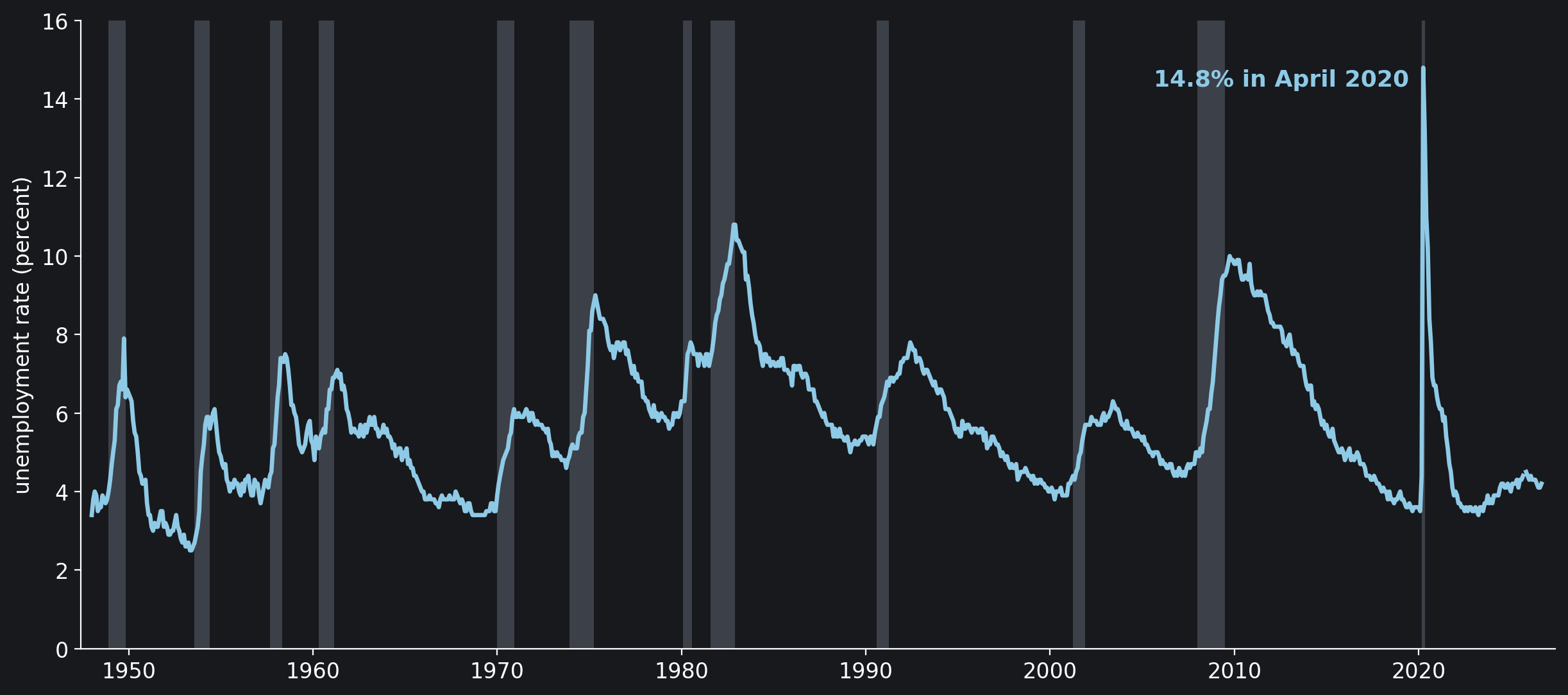
The file runs 945 months, from January 1948 to September 2026, with 944 unemployment rates. Sahm’s revised series starts in March 1949, the first month with a full year of three-month averages behind it, and has no gap; the real-time series starts in December 1959 and, like the unemployment rate, has nothing for October 2025. Figure 1 is the unemployment rate with the twelve recessions shaded: it climbs in every one of them.
The Rule, Rebuilt
With $u_t$ the unemployment rate of month $t$, the rule is two lines:
The alarm rings in month $t$ when $s_t \ge 0.50$. The first line smooths a noisy survey into a three-month average; the second measures how far that average has climbed above its best of the previous twelve months. The sentence of 2019 leaves one thing open, whether “the previous 12 months” include the current one, so the cell below builds $s_t$ with three windows and lays each beside Sahm’s own series, then works one month by hand.
The Rule, Rebuilt
m3 = u.rolling(3).mean()               # the three-month average m
windows = {"t-12 to t-1": m3.shift(1).rolling(12).min(),
           "t-12 to t": m3.rolling(13).min(),
           "t-11 to t": m3.rolling(12).min()}
for name, low in windows.items():
    both = pd.concat([(m3 - low).round(2), sahm], axis=1).dropna()
    gap = (both.iloc[:, 0] - both.iloc[:, 1]).abs().max()
    print(f"minimum over {name:<11}: {len(both)} months compared, "
          f"largest difference {gap:.2f}")

t = pd.Timestamp("2024-07-01")
last3 = u.loc[t - 2 * MONTH:t]
year = m3.loc[t - 12 * MONTH:t - MONTH]
k = year.idxmin()
print(f"\nJuly 2024: m = ({' + '.join(f'{x:.1f}' for x in last3)}) / 3 "
      f"= {m3[t]:.2f}")
print(f"lowest m of the twelve months before: {m3[k]:.2f} ({k:%B %Y})")
print(f"s = {m3[t]:.2f} - {m3[k]:.2f} = {m3[t] - m3[k]:.2f}, "
      f"Sahm's series: {sahm[t]:.2f}")

# minimum over t-12 to t-1: 919 months compared, largest difference 0.00
# minimum over t-12 to t  : 919 months compared, largest difference 0.40
# minimum over t-11 to t  : 919 months compared, largest difference 2.40
#
# July 2024: m = (3.9 + 4.1 + 4.2) / 3 = 4.07
# lowest m of the twelve months before: 3.57 (July 2023)
# s = 4.07 - 3.57 = 0.50, Sahm's series: 0.50
Over the previous twelve months, $t-12$ to $t-1$, the rebuilt gap equals Sahm’s published series to the hundredth in all 919 months where both exist; a window that includes the current month misses by up to 0.40 or 2.40 percentage points, so the rule is the one written in 2019, to the letter. July 2024 by hand: May, June and July averaged 4.07 percent, the lowest three-month average of the year before was 3.57, from July 2023, and the gap was 0.50, exactly on the line.
The Missing October
Why 919 and not 931? Sahm’s revised series has twelve more months, October 2025 to September 2026, and the strict rule cannot make them: every three-month average that touches October 2025 is missing, and each sits inside the next twelve months’ minimum. FRED’s notes for the series say nothing about the month. Its numbers say what it did: across the empty month the published series averages the months there are, so the average for October 2025 is that of August and September, $(4.3 + 4.4)/2 = 4.35$, and November’s that of September and November. The cell does the same, and nothing more; no October rate is made up.
The Missing October
# across the empty month, the mean of the months there are (two of three)
m = u.rolling(3, min_periods=2).mean().loc["1948-03":]
low = m.shift(1).rolling(12).min()     # the lowest m of t-12 to t-1
s = (m - low).round(2)                 # the gap, to the hundredth
both = pd.concat([s, sahm], axis=1).dropna()
gap = (both.iloc[:, 0] - both.iloc[:, 1]).abs().max()
print(f"{len(both)} months compared, largest difference {gap:.2f}\n")
print(f"{'month':>8}{'u':>6}{'m':>7}{'lowest m':>10}{'s':>7}{'Sahm':>7}")
for d in s.loc["2025-08":"2026-01"].index:
    rate = "" if np.isnan(u[d]) else f"{u[d]:.1f}"
    print(f"{d:%b %Y}{rate:>6}{m[d]:>7.2f}{low[d]:>10.2f}{s[d]:>7.2f}"
          f"{sahm[d]:>7.2f}")

# 931 months compared, largest difference 0.00
#
#    month     u      m  lowest m      s   Sahm
# Aug 2025   4.3   4.23      4.10   0.13   0.13
# Sep 2025   4.4   4.33      4.10   0.23   0.23
# Oct 2025         4.35      4.10   0.25   0.25
# Nov 2025   4.5   4.45      4.10   0.35   0.35
# Dec 2025   4.4   4.45      4.10   0.35   0.35
# Jan 2026   4.3   4.40      4.10   0.30   0.30
All 931 months now agree, the largest difference 0.00. The gap is kept to the hundredth, as Sahm’s series is published: the unrounded difference for October 1957 comes out of the computer as 0.49999999999999956, a hair under the line the published 0.50 sits on, and the alarm should not depend on the last digit of a binary fraction.
Every Alarm Against Every Recession
An alarm is a run of months at 0.50 or more, dated by its first month. A recession is matched with every alarm from twelve months before its peak to twelve months after its trough, the window used throughout. The months from peak to alarm are counted on the calendar, $\ell = 12\,(Y_a – Y_p) + (M_a – M_p)$: from the peak of December 2007 to the alarm of February 2008, $\ell = 12 \cdot 1 + (2 – 12) = 2$.
Every Alarm
def months(a, b):                      # calendar months from a to b
    return 12 * (b.year - a.year) + (b.month - a.month)

def alarms(x, threshold=0.5):          # the first month of each run
    on = x >= threshold
    return list(x.index[on & ~on.shift(1, fill_value=False)])

def near(t, p, tr):                    # 12 months before the peak to
    return months(p, t) >= -12 and months(tr, t) <= 12   # 12 after

first = alarms(s)
print(f"{len(first)} alarms:", ", ".join(f"{t:%b %Y}" for t in first))
print(f"\n{'peak':>8}{'trough':>10}{'alarm':>10}{'after peak':>12}"
      f"{'before trough':>15}")
for p, tr in REC:
    for t in (t for t in first if near(t, p, tr)):
        print(f"{p:%b %Y}  {tr:%b %Y}  {t:%b %Y}"
              f"{months(p, t):>+12d}{months(t, tr):>+15d}")
after = [min(months(p, t) for t in first if near(t, p, tr) and t >= p)
         for p, tr in REC]
before = [months(min(t for t in first if near(t, p, tr) and t >= p), tr)
          for p, tr in REC]
print(f"\nfirst alarm at or after each peak: {min(after)} to {max(after)}"
      f" months after it, median {np.median(after):.1f}")
print(f"months still to go to the trough: {min(before)} to {max(before)}"
      f", median {np.median(before):.1f}")

# 15 alarms: Mar 1949, Nov 1953, Oct 1957, Nov 1959, Oct 1960, Mar 1970, Jul 1974, Feb 1980, Nov 1981, Oct 1990, Jun 2001, Jul 2003, Feb 2008, Apr 2020, Jul 2024
#
#     peak    trough     alarm  after peak  before trough
# Nov 1948  Oct 1949  Mar 1949          +4             +7
# Jul 1953  May 1954  Nov 1953          +4             +6
# Aug 1957  Apr 1958  Oct 1957          +2             +6
# Apr 1960  Feb 1961  Nov 1959          -5            +15
# Apr 1960  Feb 1961  Oct 1960          +6             +4
# Dec 1969  Nov 1970  Mar 1970          +3             +8
# Nov 1973  Mar 1975  Jul 1974          +8             +8
# Jan 1980  Jul 1980  Feb 1980          +1             +5
# Jul 1981  Nov 1982  Nov 1981          +4            +12
# Jul 1990  Mar 1991  Oct 1990          +3             +5
# Mar 2001  Nov 2001  Jun 2001          +3             +5
# Dec 2007  Jun 2009  Feb 2008          +2            +16
# Feb 2020  Apr 2020  Apr 2020          +2             +0
#
# first alarm at or after each peak: 1 to 8 months after it, median 3.0
# months still to go to the trough: 0 to 16, median 6.0
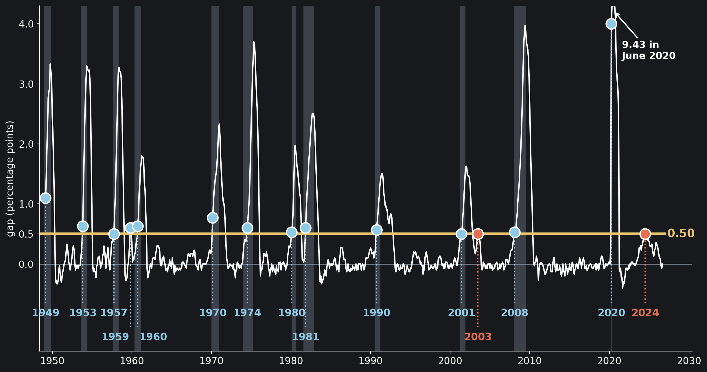
Fifteen alarms in 77 years, and every one of the twelve recessions has one. None of the twelve was foreseen: counting the first alarm at or after each peak, the rule rang 1 to 8 months after the peak, a median of 3, with 0 to 16 months of the recession still to go, a median of 6. In 2020 it rang in April, the trough itself; the recession was two months old and already over. The rule is a confirmation, not a forecast: when it rings, the recession has been under way for about a season.
It is a fast confirmation all the same. The NBER announced the December 2007 peak on 1 December 2008 and the February 2020 peak on 8 June 2020; its committee “tends to wait to identify a peak until a number of months after it has actually occurred.” Sahm’s 2019 claim was this one: the trigger “signals a recession well before the official dating of a recession.”
One alarm rang before a peak. In November 1959 the gap reached 0.60, five months before the April 1960 peak, and was back to 0.37 by January; the 1960 recession’s own alarm came in October 1960, six months after its peak. Late 1959 had a cause of its own. The Economic Report of the President of 1960 describes “the 116-day steel strike which began on July 15”: after some 500,000 steelworkers walked out, “nearly 100,000 other persons were soon laid off in related industries”, and “By the time steel production was resumed on November 7, under a Federal court injunction, employment in steel-related industries had declined by more than 500,000, exclusive of the number on strike.” Sahm counted it in 2019 as her rule’s one miss: “Earlier in the postwar period … the only false positive by this rule was in 1959, and it was followed six months later by a recession.” The window counts it as an early catch and Sahm counted it as a false alarm; either way the 1960 recession has an alarm of its own after its peak, and the medians above use that one. Figure 2 shows all fifteen.
The Alarms Without a Recession
Two alarms have no recession anywhere near them: July 2003 and July 2024. The cell follows each from two months before it to nine months after, with the unemployment rate beside the gap.
The Alarms Without a Recession
others = [t for t in first if not any(near(t, p, tr) for p, tr in REC)]
for t in others:
    run = s.loc[t:]
    end = run.index[run < 0.5][0]      # the first month back below
    prev = max(tr for p, tr in REC if tr < t)
    print(f"{t:%B %Y}: {months(prev, t)} months after the {prev:%B %Y} "
          f"trough; {months(t, end)} months at 0.50 or more, highest "
          f"{run.loc[:end].max():.2f}")
print(f"\n{'':>8}{'rate':>6}{'gap':>6}{'':>12}{'rate':>6}{'gap':>6}")
for i in range(-2, 10):
    row = ""
    for t in others:
        d = t + i * MONTH
        row += f"{d:%b %Y}{u[d]:>6.1f}{s[d]:>6.2f}" + " " * 4
    print(row.rstrip())
after24 = s.loc["2024-10":]
print(f"\nsince October 2024: highest gap {after24.max():.2f}, "
      f"in {after24.idxmax():%B %Y}; September 2026: {s.iloc[-1]:.2f}")

# July 2003: 20 months after the November 2001 trough; 2 months at 0.50 or more, highest 0.50
# July 2024: 51 months after the April 2020 trough; 3 months at 0.50 or more, highest 0.57
#
#           rate   gap              rate   gap
# May 2003   6.1  0.30    May 2024   3.9  0.40
# Jun 2003   6.3  0.43    Jun 2024   4.1  0.43
# Jul 2003   6.2  0.50    Jul 2024   4.2  0.50
# Aug 2003   6.1  0.50    Aug 2024   4.2  0.57
# Sep 2003   6.1  0.43    Sep 2024   4.1  0.53
# Oct 2003   6.0  0.37    Oct 2024   4.1  0.40
# Nov 2003   5.8  0.20    Nov 2024   4.2  0.40
# Dec 2003   5.7 -0.03    Dec 2024   4.1  0.40
# Jan 2004   5.7 -0.10    Jan 2025   4.0  0.37
# Feb 2004   5.6 -0.07    Feb 2025   4.2  0.30
# Mar 2004   5.8  0.03    Mar 2025   4.2  0.30
# Apr 2004   5.6  0.00    Apr 2025   4.2  0.30
#
# since October 2024: highest gap 0.40, in October 2024; September 2026: 0.00
The 2003 alarm came 20 months after the November 2001 trough, with the unemployment rate still rising, to 6.3 percent in June 2003, the highest it reached after that recession. It lasted two months at exactly 0.50 and was gone by September. Sahm’s 2019 sentence, “only during or closely following recessions”, has room for it.
July 2024 has no such room: the last trough was April 2020, more than four years before. The alarm lasted three months, July to September 2024, and peaked at 0.57 in August; the gap was back to 0.40 in October, has not been higher since, and reads 0.00 in September 2026. Sahm’s explanation, in Stay-At-Home Macro on 6 September 2024: “There are signs that stronger labor supply, not just weaker labor demand, helped push the Sahm rule past its 0.50 percentage point threshold.” “Unemployed entrants to the labor force (new or returning) accounted for about half of the increase.” Hence “The current Sahm rule reading is likely overstating the weakening in demand and not at recessionary levels,” because “The Sahm rule does not distinguish between these two dynamics, and can look more ominous when the labor force is expanding rapidly.” On 10 February 2026, after the revised payroll figures, she added: “July 2024 was also when the rise in the unemployment rate triggered the Sahm rule recession indicator. At the time, the unemployment rate appeared out of step with payrolls, but that gap largely reflected the long lags in measuring employment.”
As of September 2026, the last month in the file, the NBER has dated no recession since 2020: its business-cycle page still reads “The most recent trough occurred in April 2020,” and the committee’s latest announcement, of 19 July 2021, is the determination of that trough.
Real Time Against Revised
Everything so far uses today’s data, which nobody had at the time. In FRED’s words, SAHMREALTIME “is based on “real-time” data, that is, the unemployment rate (and the recent history of unemployment rates) that were available in a given month”, and “The BLS revises the unemployment rate each year at the beginning of January, when the December unemployment rate for the prior year is published.” The cell sets the indicator as it was published against today’s, month by month and alarm by alarm, from 1960.
Real Time Against Revised
rt = df["SAHMREALTIME"]                # the indicator as first published
both = pd.concat([rt.rename("then"), s.rename("now")], axis=1).dropna()
diff = (both["then"] - both["now"]).round(2)
print(f"{len(both)} months with both; identical in {(diff == 0).mean():.0%}"
      f", mean gap {diff.abs().mean():.2f}; largest:")
for d in diff.abs().nlargest(4, keep="first").index:
    print(f"  {d:%b %Y}: then {both.then[d]:.2f}, now {both.now[d]:.2f}")
for d in pd.to_datetime(["2003-07-01", "2024-07-01"]):
    print(f"{d:%B %Y}: then {both.then[d]:.2f}, now {both.now[d]:.2f}")
sides = ((both.then >= 0.5) != (both.now >= 0.5)).sum()
print(f"months on opposite sides of 0.50: {sides}")

then_ = [t for t in alarms(rt) if t.year >= 1960]
now_ = [t for t in first if t.year >= 1960]
print(f"\n{'peak':>8}{'alarm then':>16}{'alarm now':>16}")
lag = {"then": [], "now": []}
for p, tr in REC[3:]:
    row = f"{p:%b %Y}"
    for key, runs in (("then", then_), ("now", now_)):
        t = next(t for t in runs if near(t, p, tr))
        lag[key].append(months(p, t))
        row += f"{t:%b %Y}".rjust(12) + f"{months(p, t):>+4d}"
    print(row)
for key, runs in (("then", then_), ("now", now_)):
    lone = [t for t in runs if not any(near(t, p, tr) for p, tr in REC)]
    print(f"{key}: median {np.median(lag[key]):.0f} months after the peak;"
          f" no recession near: {', '.join(f'{t:%b %Y}' for t in lone)}")

# 801 months with both; identical in 27%, mean gap 0.05; largest:
#   Nov 1976: then 0.50, now 0.13
#   Oct 1960: then 0.93, now 0.63
#   Oct 1976: then 0.43, now 0.13
#   Nov 1960: then 1.07, now 0.80
# July 2003: then 0.47, now 0.50
# July 2024: then 0.53, now 0.50
# months on opposite sides of 0.50: 16
#
#     peak      alarm then       alarm now
# Apr 1960    Aug 1960  +4    Oct 1960  +6
# Dec 1969    Oct 1969  -2    Mar 1970  +3
# Nov 1973    Mar 1974  +4    Jul 1974  +8
# Jan 1980    Apr 1980  +3    Feb 1980  +1
# Jul 1981    Nov 1981  +4    Nov 1981  +4
# Jul 1990    Nov 1990  +4    Oct 1990  +3
# Mar 2001    Jun 2001  +3    Jun 2001  +3
# Dec 2007    Apr 2008  +4    Feb 2008  +2
# Feb 2020    Apr 2020  +2    Apr 2020  +2
# then: median 4 months after the peak; no recession near: Nov 1976, Jul 2024
# now: median 3 months after the peak; no recession near: Jul 2003, Jul 2024
The two series agree to the hundredth in 27% of the 801 months they share and differ by 0.05 on average. July 2024 read 0.53 as published and reads 0.50 today, still on the line, by a hair. The largest gaps are older: November 1976 read 0.50 then and reads 0.13 now, October 1960 0.93 then and 0.63 now.
Run on what was known at the time, the alarm rang for each of the nine recessions since 1960, a median of 4 months after the peak, against 3 on today’s data. It is not a fixed delay: real time was earlier in 1960 and 1973, later in 1980, 1990 and 2008, and in 1969 it rang in October, two months before the December peak. The six real-time alarms for the recessions since 1970 are the six months Sahm’s 2019 chapter drew in its figure 3: March 1974, April 1980, November 1981, November 1990, June 2001 and April 2008. The alarms without a recession change too. In real time the rule never rang in 2003 (0.47 in July 2003), but it rang in November 1976, twenty months after the March 1975 trough, which today’s data put at 0.13. Each version has two alarms with no recession near, and only one of them is the same: July 2024.
Every Threshold
Sahm chose 0.50 in 2019. The cell runs the alarm at five thresholds, with the same window.
Every Threshold
def score(threshold):
    runs = alarms(s, threshold)
    caught = sum(any(near(t, p, tr) for t in runs) for p, tr in REC)
    lone = [t for t in runs if not any(near(t, p, tr) for p, tr in REC)]
    return runs, caught, lone

print(f"{'threshold':>9}{'alarms':>8}{'recessions caught':>19}"
      f"{'no recession near':>19}")
for th in (0.3, 0.4, 0.5, 0.6, 0.7):
    runs, caught, lone = score(th)
    print(f"{th:>9.2f}{len(runs):>8}{f'{caught} of {len(REC)}':>19}"
          f"{len(lone):>19}")

# threshold  alarms  recessions caught  no recession near
#      0.30      22           12 of 12                  7
#      0.40      16           12 of 12                  2
#      0.50      15           12 of 12                  2
#      0.60      13           12 of 12                  0
#      0.70      13           12 of 12                  1
Every threshold from 0.30 to 0.70 catches all twelve recessions; what changes is the alarms with none. At 0.30 there are seven, at 0.40 and 0.50 two, at 0.70 one (June 1992, fifteen months after the March 1991 trough), and at 0.60 none: set at 0.60, the rule has never rung with no recession near since 1949 (the 1959 strike month, at exactly 0.60, still rings, inside the 1960 window). Choosing 0.60 after seeing these 77 years is hindsight, a threshold fitted to the twelve recessions already known and to the 2003 and 2024 alarms it was picked to miss.
Your Own Threshold
Put any threshold at the top of the cell and run it (0.3 to 0.7 is the useful range). It prints the alarms with no recession near, and for each recession the first alarm inside its window, counted from the peak: a minus sign means it rang before the peak.
Your Own Threshold
THRESHOLD = 0.5                        # try anything from 0.3 to 0.7

runs, caught, lone = score(THRESHOLD)
print(f"threshold {THRESHOLD:.2f}: {len(runs)} alarms, {caught} of "
      f"{len(REC)} recessions caught, {len(lone)} with no recession near")
for t in lone:
    print(f"  no recession near: {t:%B %Y}")
lags = [months(p, t) for p, tr in REC
        for t in [t for t in runs if near(t, p, tr)][:1]]
print("each recession's first alarm, months from its peak:",
      " ".join(f"{x:+d}" for x in lags))
print(f"median {np.median(lags):+.1f} months")

# threshold 0.50: 15 alarms, 12 of 12 recessions caught, 2 with no recession near
#   no recession near: July 2003
#   no recession near: July 2024
# each recession's first alarm, months from its peak: +4 +4 +2 -5 +3 +8 +1 +4 +3 +3 +2 +2
# median +3.0 months
At 0.50 the cell gives back the table above with the 1959 strike alarm in its place, −5 for the 1960 recession, and the median stays at 3 months after the peak. Lower the threshold and the alarm rings earlier: at 0.30 the median is 1 month after the peak and four of the twelve recessions are flagged before it, at the price of seven alarms with no recession near. Raise it and it rings later: a median of 4 months at 0.60, 4.5 at 0.70.
What the Numbers Show
Has the Sahm rule ever been wrong? Rebuilt to the letter from the unemployment rate, it matches Sahm’s published series in all 931 months, and it rang in every one of the twelve recessions since 1948, a median of 3 months after the peak. It rang three times without one under way: in late 1959, during the steel strike, five months before a recession that came anyway; in July 2003, twenty months into a recovery with unemployment still rising; and in July 2024, with no recession on either side. On the data published at the time the list is different, 1976 instead of 2003, but July 2024 is on both, at 0.53 then and 0.50 now. July 2024 is the rule’s one clean miss in 77 years: it rang on a rise in unemployment of which, by Sahm’s own count, about half came from people entering the labor force, and no recession followed.
Five limits, each in one sentence. The rule is a confirmation, not a forecast: in all twelve recessions it rang after the peak. The revised series is not what anyone saw at the time, which is what SAHMREALTIME is for, and the two disagree about which alarms were false. Twelve recessions are a small sample for any rule. A threshold tuned on them, such as the 0.60 that leaves no alarm without a recession near, is hindsight. And “no recession since 2020” holds as of September 2026, the last month in the file; the NBER dates recessions with a long delay, so a recession under way in 2026 would not be dated yet.
Sources
- C. Sahm, “Direct Stimulus Payments to Individuals”, chapter 3 of Recession Ready: Fiscal Policies to Stabilize the American Economy (The Hamilton Project, 16 May 2019), pages 67–92: the rule, its test on real-time data since 1970, and endnote 7 on 1959.
- C. Sahm, Stay-At-Home Macro: “Sahm-thing more on the Sahm rule” (26 July 2024), “Labor market conditions.” (6 September 2024) and “A Year With No Jobs—But No Recession” (10 February 2026).
- FRED, Federal Reserve Bank of St. Louis: U.S. Bureau of Labor Statistics, Unemployment Rate [UNRATE]; Claudia Sahm, Sahm Rule Recession Indicator [SAHMCURRENT]; Claudia Sahm, Real-time Sahm Rule Recession Indicator [SAHMREALTIME]; retrieved 16 October 2026, with their series notes. Each is marked public domain, citation requested.
- U.S. Bureau of Labor Statistics, “2025 federal government shutdown impact on the Current Population Survey” (last modified 11 March 2026).
- National Bureau of Economic Research, “US Business Cycle Expansions and Contractions”, the Business Cycle Dating page and the committee’s announcements.
- Economic Report of the President, 1960, chapter 2, “Economic Developments in 1959”, via FRASER, Federal Reserve Bank of St. Louis: the 1959 steel strike.
Every number in this notebook is computed by its own cells from the one data file.
Interested in applying these ideas to your work? Get in touch.
Also on
 YouTubeHas the Sahm Rule Ever Been Wrong? Every Recession Alarm Since 1949 in PythonThis notebook in plain words, in a few minutes.Watch on YouTube →FacebookThe walkthrough on our Facebook PageThe short film, with its comments.Discuss on Facebook →The same notebook on KaggleRun it in the browser, cell by cell, on Kaggle.Run the notebook →