Hawkes Process Models for High-Frequency Trade Arrivals

1. Introduction

In modern electronic markets, trades and quote updates do not arrive at a constant rate. Following a large print, a cascade of aggressive orders, cancellations, and responses from algorithmic market-makers typically erupts within milliseconds. This clustering of events is one of the most robust stylised facts of high-frequency financial data. The Hawkes process, introduced by Alan Hawkes in 1971, is a self-exciting point process that models this behaviour directly: each event transiently raises the probability of further events, with the excitation decaying over time.

Applications in finance include modelling trade arrivals, bid-ask spread dynamics, price impact, and the propagation of volatility shocks across assets and venues.

2. The Univariate Hawkes Process

Let N(t) be a counting process on \lbrack 0,\infty). It is a Hawkes process if its \mathcal{F}_t-conditional intensity takes the form

where \mu \gt 0 is the baseline intensity and \varphi : \mathbb{R}_+ \to \mathbb{R}_+ is the excitation kernel, quantifying how much each past event raises the current intensity.

The most widely used kernel is the exponential kernel,

where \alpha controls the jump size at each event and \beta controls the decay rate. The branching ratio

is the expected number of events triggered by a single event. Stationarity requires n \lt 1; values close to 1 correspond to highly clustered, near-critical processes.

3. Multivariate Extension

In practice, order arrivals on the bid and ask sides of the book are not independent. A multivariate Hawkes process on d components has intensity vector

The kernel matrix \Phi = (\varphi^{kj}) encodes both self-excitation (diagonal, k = j) and cross-excitation (off-diagonal, k \neq j). A symmetric two-dimensional Hawkes process on upward and downward price moves reproduces the Epps effect and the signature plot of realised volatility.

4. Likelihood Estimation

Given observed event times t_1 \lt t_2 \lt \cdots \lt t_n on \lbrack 0, T\rbrack, the log-likelihood is

This is evaluated in O(n) time via the recursion R_i = e^{-\beta(t_i - t_{i-1})}(1 + R_{i-1}) with R_1 = 0, so \sum_{j \lt i} e^{-\beta(t_i - t_j)} = R_i. MLE proceeds via standard gradient-based optimisers.

5. Simulated Example

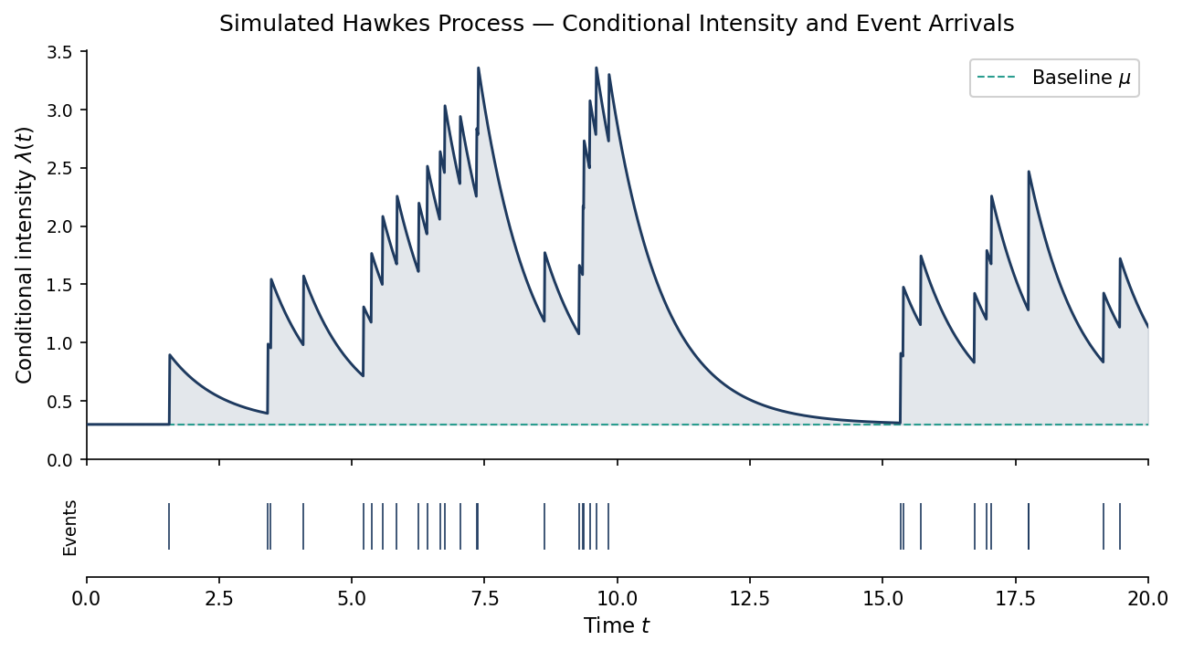
The following code simulates a univariate Hawkes process with exponential kernel using Ogata’s thinning algorithm, then plots the conditional intensity alongside the event arrival times.

import numpy as np
import matplotlib.pyplot as plt

np.random.seed(42)

# Parameters
mu, alpha, beta, T = 0.3, 0.6, 1.0, 20.0

# Ogata thinning simulation
events = []
t = 0.0
while t < T:
    lam = mu + sum(alpha * np.exp(-beta * (t - ti)) for ti in events)
    t  += np.random.exponential(1.0 / lam)
    if t > T:
        break
    lam_new = mu + sum(alpha * np.exp(-beta * (t - ti)) for ti in events)
    if np.random.uniform() < lam_new / lam:
        events.append(t)

events = np.array(events)

# Compute intensity on fine grid
tgrid     = np.linspace(0, T, 2000)
intensity = np.array([mu + sum(alpha * np.exp(-beta * (t - ti))
                      for ti in events if ti < t) for t in tgrid])

# Plot
fig, (ax1, ax2) = plt.subplots(2, 1, figsize=(10, 5), sharex=True,
                    gridspec_kw={'height_ratios': [4, 1], 'hspace': 0.06})

ax1.plot(tgrid, intensity, color='#1e3a5f', lw=1.4)
ax1.axhline(mu, color='#2a9d8f', lw=1.0, ls='--', label=r'Baseline $\mu$')
ax1.fill_between(tgrid, mu, intensity, alpha=0.12, color='#1e3a5f')
ax1.set_ylabel(r'Conditional intensity $\lambda(t)$', fontsize=11)
ax1.set_ylim(0, None)
ax1.legend(fontsize=10, framealpha=0.9)
ax1.set_title('Simulated Hawkes Process', fontsize=12, pad=10)
ax1.spines['top'].set_visible(False)
ax1.spines['right'].set_visible(False)

ax2.eventplot(events, orientation='horizontal', colors='#1e3a5f',
              lineoffsets=0.5, linelengths=0.8, lw=0.8)
ax2.set_xlabel('Time $t$', fontsize=11)
ax2.set_yticks([])
ax2.set_xlim(0, T)
for sp in ['top', 'right', 'left']:
    ax2.spines[sp].set_visible(False)

plt.savefig('hawkes_hf.png', dpi=150, bbox_inches='tight', facecolor='white')

The figure below shows the output: the upper panel traces \lambda(t), which spikes at each event and decays exponentially back to \mu; the lower panel marks event arrival times.

6. Empirical Stylised Facts

When calibrated to trade-by-trade data on liquid equity futures, the Hawkes model reproduces several key stylised facts:

• Clustering and bursts. The branching ratio typically lies in \lbrack 0.5, 0.95\rbrack, implying most trades are endogenously triggered rather than driven by exogenous information.
• Power-law autocorrelation. Mixtures of exponentials approximate power-law memory, consistent with long-range dependence in trade-count autocorrelations.
• Intraday seasonality. The baseline \mu(t) can be made time-varying to absorb the U-shaped intraday activity pattern.
• Price diffusion. In the symmetric bivariate model, mid-price variance grows linearly at long horizons, consistent with efficient market behaviour.

References

1. Hawkes, A. G. (1971). Spectra of some self-exciting and mutually exciting point processes. Biometrika, 58(1), 83–90.
2. Bacry, E., Mastromatteo, I., & Muzy, J.-F. (2015). Hawkes processes in finance. Market Microstructure and Liquidity, 1(1), 1550005.
3. Bowsher, C. G. (2007). Modelling security market events in continuous time. Journal of Econometrics, 141(2), 876–912.
4. Embrechts, P., Liniger, T., & Lin, L. (2011). Multivariate Hawkes processes: An application to financial data. Journal of Applied Probability, 48(A), 367–378.
5. Bacry, E., & Muzy, J.-F. (2014). Hawkes model for price and trades high-frequency dynamics. Quantitative Finance, 14(7), 1147–1166.