Pricing a Gas Liquefaction Plant as a Real Option: An HJB Approach

The Limits of Static NPV

Infrastructure investment decisions are rarely simple discounted cash flow problems. When you are considering a multi-billion dollar capital commitment whose returns depend on a volatile commodity price over a twenty-five year horizon, static NPV analysis misses the most economically important feature of the decision: **you can wait**.

The option to delay is not free. Every year you wait is a year of cash flows forgone. But exercising the option prematurely — investing before the price environment justifies it — destroys value just as surely. This trade-off is precisely the structure that **real options theory** is built to handle, and the **Hamilton-Jacobi-Bellman (HJB) equation** is the correct mathematical framework for pricing it.

In this post, we set up the HJB equations in their full form, show how they reduce to tractable linear PDEs, and then solve them numerically to derive the optimal investment threshold as a function of time.

The Project

We consider a single LNG liquefaction train — a facility that processes raw natural gas into liquid LNG for export. The parameters below are representative of a mid-size Gulf facility.

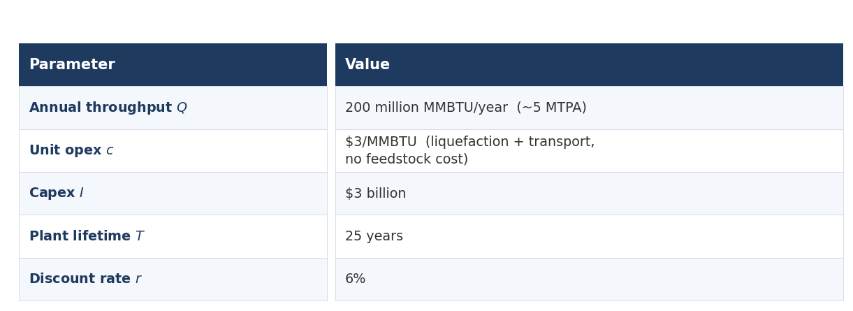
We assume **stranded gas** — the feedstock cost is negligible, as is the case for Qatar’s North Field. The plant has two decision makers: an **operator** who controls day-to-day running, and an **investor** who decides when (or whether) to build it.

Gas Price Dynamics: The CIR Process

We model the gas price $S_t$ under the risk-neutral measure as a **Cox-Ingersoll-Ross (CIR) process**:

The parameters are calibrated to monthly TTF/Henry Hub data (monthly averaging smooths out daily noise irrelevant to plant-level decisions):

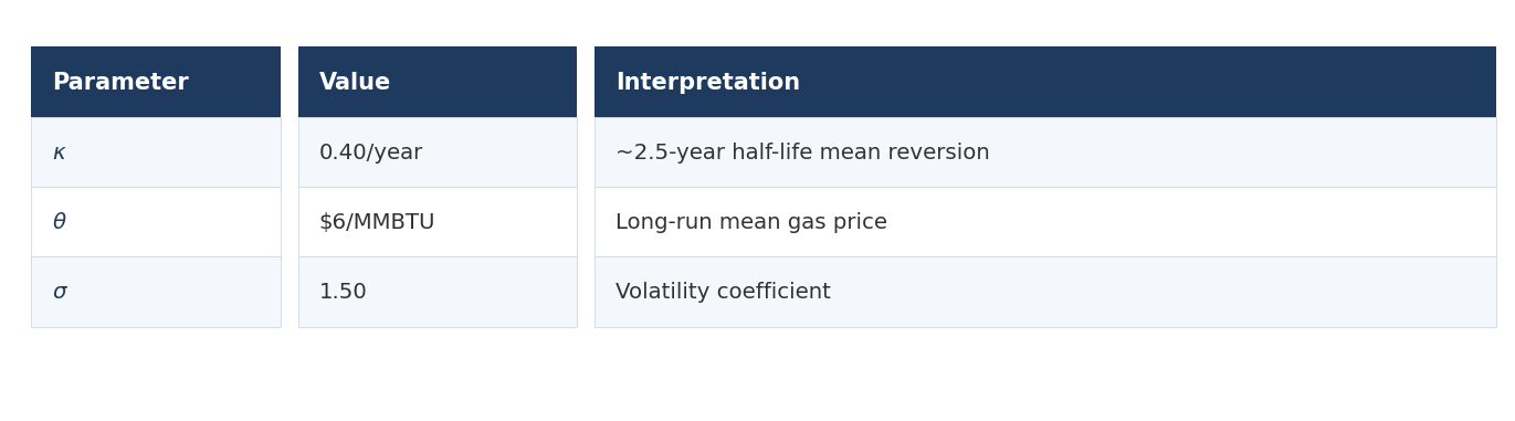
The CIR process has two properties that matter here. First, $S_t \geq 0$ always (the Feller condition $\sigma^2 \leq 2\kappa\theta$ holds with these parameters). Second, mean reversion reflects genuine gas market economics: supply responds to sustained high prices over months to years, pulling prices back toward long-run marginal cost.

The square-root diffusion gives the process **level-dependent volatility** — a 1 USD shock matters more at $S =$ 3 USD than at $S =$ 15 USD, which matches observed price dynamics.

The Two Value Functions

We work with two value functions that correspond to the two decision makers:

**$W(S, t)$** — the value of the plant to its owner, *after* the investment has been made. At each instant the operator chooses whether to run or idle. $t$ counts years elapsed; the plant runs from $t = 0$ to $t = T$.

**$V(S, t)$** — the value of the *option to invest*, before committing the capex. The investor can build the plant at any time up to $T$ by paying $I$, after which they receive $W$.

Both value functions depend on the current gas price $S$ and time $t$. The question is: what PDEs do they satisfy, and where do they come from?

The Full HJB Equations

The operating plant: a stochastic control problem

The operator controls a binary variable $u_t \in \{0, 1\}$ — run ($u=1$) or idle ($u=0$) — at each instant. Running yields revenue $Q(S_t – c)$ per year; idling yields zero. The operator maximises the expected discounted cumulative profit:

$$W(S, t) = \sup_{\{u_s\}_{s \geq t}} \mathbb{E}\!\left[\int_t^T e^{-r(s-t)} u_s \cdot Q(S_s – c)\,ds \;\Big|\; S_t = S\right]$$

By the dynamic programming principle, $W$ satisfies the **HJB equation**:

The supremum in equation (2) is the HJB nonlinearity. It reflects the operator’s optimal choice at every point $(S, t)$.

Resolving the supremum in closed form

The supremum $\sup_{u \in \{0,1\}}\{u \cdot Q(S-c)\}$ is maximised over a two-element set. Since $Q > 0$, the optimal control is:

$$u^*(S) = \begin{cases} 1 & \text{if } S > c \\ 0 & \text{if } S \leq c \end{cases}$$

Run when the gas price exceeds unit opex; idle otherwise. Substituting back:

$$\sup_{u \in \{0,1\}}\bigl\{u \cdot Q(S-c)\bigr\} = Q\max(S – c,\; 0) \;\equiv\; \pi(S)$$

This is exact — not an approximation. The nonlinear sup collapses to a fixed, known function of $S$ alone, because the control enters linearly and the control set is finite. Equation (2) becomes the **linear PDE**:

with terminal condition $W(S, T) = 0$, boundary condition $W(0, t) = 0$, and a Neumann condition at $S_{\max}$. The operating option is already embedded in $\pi(S) = Q\max(S-c, 0)$: the plant idles when $S < c =$ 3 USD/MMBTU, incurring zero loss rather than a negative cash flow.

The investment option: an optimal stopping problem

The investor holds an American-style real option: pay $I$ at any time $\tau \leq T$ and receive the operating plant value $W(S_\tau, \tau)$. The investor chooses $\tau$ to maximise the expected discounted payoff:

$$V(S, t) = \sup_{\tau \in [t, T]} \mathbb{E}\!\left[e^{-r(\tau – t)}\bigl(W(S_\tau, \tau) – I\bigr)^+ \;\Big|\; S_t = S\right]$$

For optimal stopping problems, the dynamic programming principle gives not a PDE but a **variational inequality** — the full HJB in this setting:

The min operator encodes the two-region structure of the optimal stopping problem simultaneously.

Resolving the variational inequality: two regions

Equation (4) implies that at every point $(S, t)$, exactly one of two conditions holds:

**Continuation region** — where waiting is strictly optimal: $V(S, t) > W(S, t) – I$. The second argument of the min is positive, so the first must be zero:

This is a **linear PDE** — structurally identical to the Black-Scholes equation with the CIR generator in place of the GBM generator.

**Exercise region** — where investing immediately is optimal: $V(S, t) = W(S, t) – I$. The first argument of the min is positive (or zero), and the obstacle constraint is binding.

The curve $S^*(t)$ separating these regions is the **free boundary** — the minimum gas price at which it is optimal to invest today given $t$ years elapsed. It is not imposed; it emerges from the solution.

Boundary conditions at the free boundary

At $S^*(t)$, continuity of $V$ and its derivative are required. These are the **value-matching** and **smooth-pasting** conditions:

The smooth-pasting condition (equation (7)) is a necessary condition for optimality: if the derivative of $V$ were discontinuous at $S^*(t)$, the investor could do strictly better by adjusting the threshold slightly, contradicting optimality.

Numerical Solution

We now have two linear parabolic PDEs — equations (3) and (5) — on the same $(S, t)$ grid, coupled through the obstacle constraint. We solve them by **backward induction**, starting from $t = T$ and stepping backward.

The spatial grid runs from $S = 0$ to $S_{\max} =$ 25 USD/MMBTU with $M = 400$ points ($\Delta S =$ 0.0625 USD). Time is discretised into $N = 2000$ steps ($\Delta t = 0.0125$ years ≈ 4.6 days). A **fully implicit** finite difference scheme is used for stability under the CIR diffusion, whose coefficient $\frac{1}{2}\sigma^2 S$ vanishes at $S = 0$.

At each backward step, we:

• Advance $W^{n+1}$ from $W^n$ by solving a tridiagonal system with the CIR generator and profit term $\pi(S)$.
• Advance $V^{n+1}$ from $V^n$ using the same tridiagonal matrix but no profit term.
• Apply the obstacle projection: $V^{n+1} = \max(V^{n+1}, W^{n+1} – I)$. This enforces the variational inequality (4) at the discrete level.
• Identify the free boundary $S^*(t)$ as the lowest $S$ where the obstacle constraint is binding.

import numpy as np
from scipy.linalg import solve_banded

# ── Shared parameters ──────────────────────────────────────────────────────────
kappa, theta, sigma = 0.40, 6.00, 1.50   # CIR: same for HJB and simulation
r, T, Q  = 0.06, 25.0, 200e6
c_unit, I = 3.00, 3.0e9

# ── HJB grid ───────────────────────────────────────────────────────────────────
S_max, M, N = 25.0, 400, 2000
dS, dt = S_max / M, T / N
S    = np.linspace(0.0, S_max, M + 1)
pi_S = Q * np.maximum(S - c_unit, 0.0)

# Fully implicit tridiagonal coefficients
alpha = 0.5 * sigma**2 * S / dS**2
beta  = kappa * (theta - S) / (2.0 * dS)
lo    = -(alpha - beta) * dt
mid   =  1.0 + (2.0 * alpha + r) * dt
hi    = -(alpha + beta) * dt

Ab = np.zeros((3, M + 1))
Ab[0, 1:]  = hi[:-1];   Ab[1, :] = mid;   Ab[2, :-1] = lo[1:]
Ab[1, 0]   = 1.0;       Ab[0, 1] = 0.0                     # BC S=0
Ab[1, M]   = 1.0;       Ab[2, M-1] = -1.0                  # BC Neumann

# ── Backward induction ─────────────────────────────────────────────────────────
W, V = np.zeros(M + 1), np.zeros(M + 1)
free_bdry = []   # (t_remaining, S_star)

for n in range(N):
    rhs = W + pi_S * dt;  rhs[0] = rhs[M] = 0.0
    W   = np.maximum(solve_banded((1,1), Ab, rhs), 0.0)

    rhs_v = V.copy();  rhs_v[0] = rhs_v[M] = 0.0
    V = np.maximum(solve_banded((1,1), Ab, rhs_v), 0.0)
    V = np.maximum(V, W - I)   # obstacle projection — enforces eq. (4)

    idx = np.where((W - I) > V - 1e3)[0]
    free_bdry.append(((n + 1) * dt, S[idx[0]] if len(idx) else S_max))

free_bdry = np.array(free_bdry)   # col0 = t_remaining, col1 = S*

# ── CIR sample path — Euler-Maruyama (continuous time, annual parameters) ──────
rng      = np.random.default_rng(7)
n_sim    = 5000
dt_sim   = T / n_sim
S_cir    = np.zeros(n_sim + 1)
S_cir[0] = 4.5   # start below threshold

for i in range(n_sim):
    s           = max(S_cir[i], 0.0)
    dW          = rng.normal(0.0, np.sqrt(dt_sim))
    S_cir[i+1]  = max(s + kappa*(theta - s)*dt_sim + sigma*np.sqrt(s)*dW, 0.0)

# ── First exercise: map threshold to elapsed-time axis ─────────────────────────
t_elapsed     = np.linspace(0.0, T, n_sim + 1)   # years elapsed (x-axis)
t_elap_bdry   = T - free_bdry[:, 0]              # remaining → elapsed
sort_idx      = np.argsort(t_elap_bdry)
threshold_sim = np.interp(t_elapsed,
                          t_elap_bdry[sort_idx],
                          free_bdry[sort_idx, 1])

above   = S_cir >= threshold_sim
hit_idx = int(np.argmax(above)) if np.any(above) else None
# hit_idx is the first time step where the CIR path crosses the threshold

The Investment Threshold

The key output is the **free boundary** $S^*(t)$ — the minimum gas price at which it is optimal to commit the 3 billion USD capex today, given $t$ years elapsed into the plant’s 25-year life.

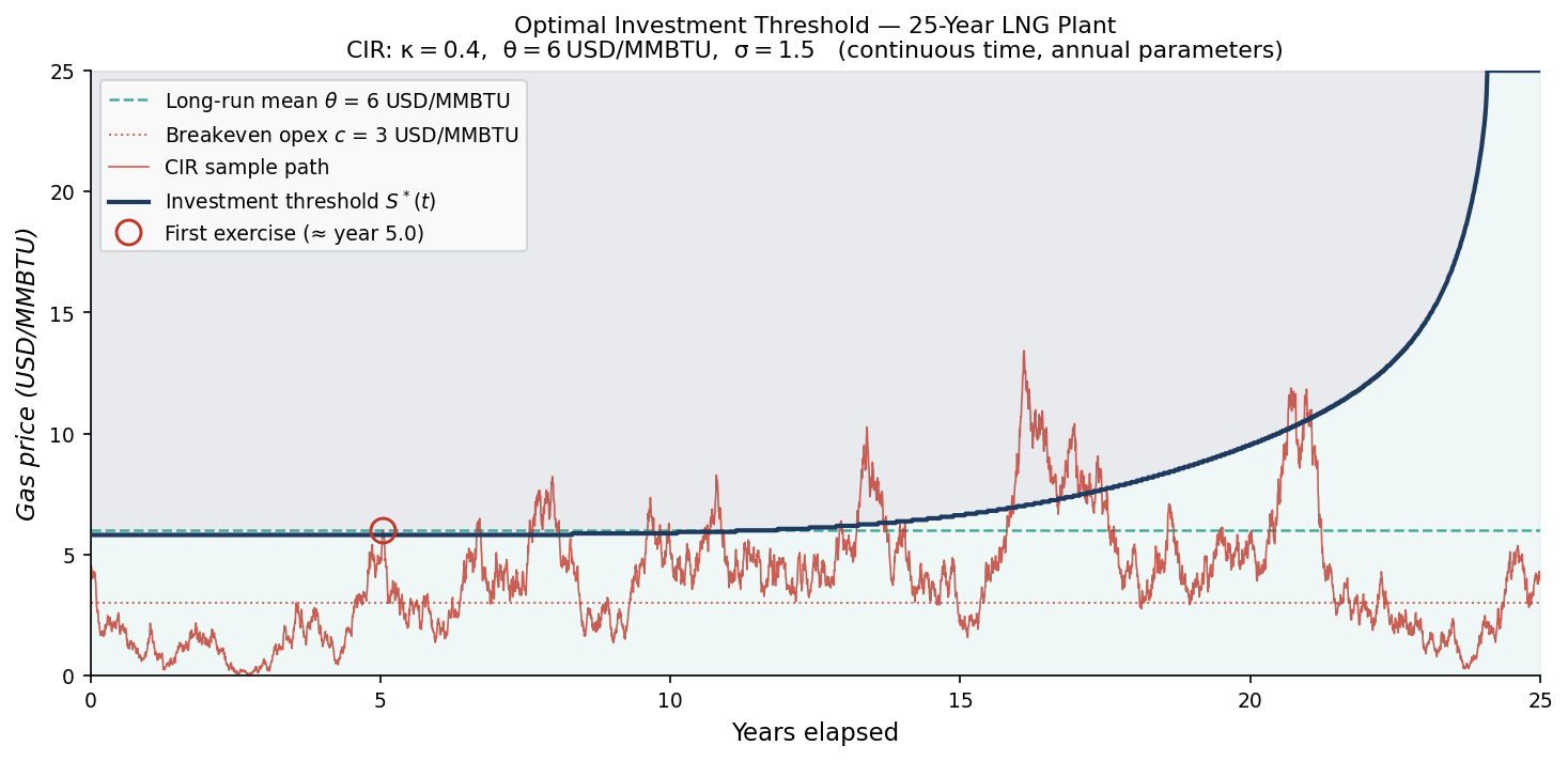
The figure shows a representative realisation of the CIR process starting at 4.5 USD/MMBTU — firmly below the threshold at project inception. For roughly five years the price meanders below the threshold, mean-reverting toward 6 USD/MMBTU. At approximately year five the path first rallies to meet the threshold: this is the optimal moment to commit the 3 billion USD capex for this particular price history. An investor who had acted at year zero, when the price was below the threshold, would have sacrificed option value unnecessarily. One who waited beyond the first crossing would have continued holding an option that had already become worth zero — the continuation value equals the immediate payoff.

Several features of the threshold itself are immediately apparent:

**The threshold starts near the long-run mean and rises steeply.** At project inception (year 0, full 25-year horizon), the threshold is close to 6 USD/MMBTU — near the long-run mean $\theta$. This is above the static NPV break-even of roughly 4.2 USD/MMBTU: the premium is the **value of waiting**, which compensates for giving up the option to invest later at a more favourable price.

**The threshold rises as time runs out.** As the remaining horizon shrinks, the window for recovering the 3 billion USD capex narrows sharply. In the final years, the threshold climbs toward infinity: it is almost never rational to invest when only months of plant life remain.

**The long-run limit.** As the time horizon lengthens, $S^*(t)$ converges toward a steady-state value $S^{**}$ — the threshold for the **perpetual plant** problem, discussed below.

The Infinite Horizon Limit

When $T \to \infty$, the problem becomes time-homogeneous and $V(S, t) = V(S)$, $W(S, t) = W(S)$. The PDEs (3) and (5) degenerate to a system of **ordinary differential equations**:

These ODEs can be solved semi-analytically using confluent hypergeometric functions, and the threshold $S^{**}$ is determined by the smooth-pasting conditions. The finite-horizon free boundary $S^*(t)$ converges to $S^{**}$ from above as the horizon grows — visible in the figure as the asymptote at the left edge.

This reduction is useful for sensitivity analysis: the ODE system is fast to solve and allows rapid calibration to different gas price scenarios.

What the Numbers Say

At current European TTF spot prices around 8–10 USD/MMBTU (mid-2024 levels), the model suggests that a well-capitalised investor **would be near or above the investment threshold** for a 25-year plant. At $S =$ 9 USD, with 20 years of plant life, the operating value $W \approx$ 6.5 billion USD against a 3 billion USD capex outlay — a net payoff of 3.5 billion USD that comfortably clears the smooth-pasting condition.

At $S =$ 5 USD — the Henry Hub neighbourhood — the investment is firmly in the continuation region. The option value $V$ reflects the probability of a future price spike bringing the project into the exercise region.

The model also prices the **idle option** embedded in the plant operations. By allowing the plant to shut down when $S <$ 3 USD/MMBTU, we add approximately 400 million USD to the operating value compared to a plant that must run continuously — a meaningful correction that pure DCF would miss.

Takeaway

The HJB framework forces you to answer the question that NPV glosses over: not whether to invest, but **at what price, and how urgently**. Starting from the full HJB equations — one for the operating control problem, one for the optimal stopping problem — both nonlinearities resolve cleanly: the bang-bang operating control becomes $\pi(S) = Q\max(S-c,0)$, and the variational inequality splits into a linear PDE in the continuation region plus an obstacle constraint at the free boundary. What remains is two coupled linear parabolic PDEs, solvable by standard backward induction.

For a project of this scale and duration, the gap between the static NPV break-even and the optimal exercise threshold is several USD per MMBTU. Getting that number right is not an academic exercise — it is the difference between committing 3 billion USD at the wrong time and waiting for an environment that genuinely justifies the risk.

Working on a pricing model or risk system? Let’s talk.