Kelly, the Growth-Optimal Portfolio, and the Benchmark Approach to Option Pricing
From Coin Flips to Risk-Neutral Pricing
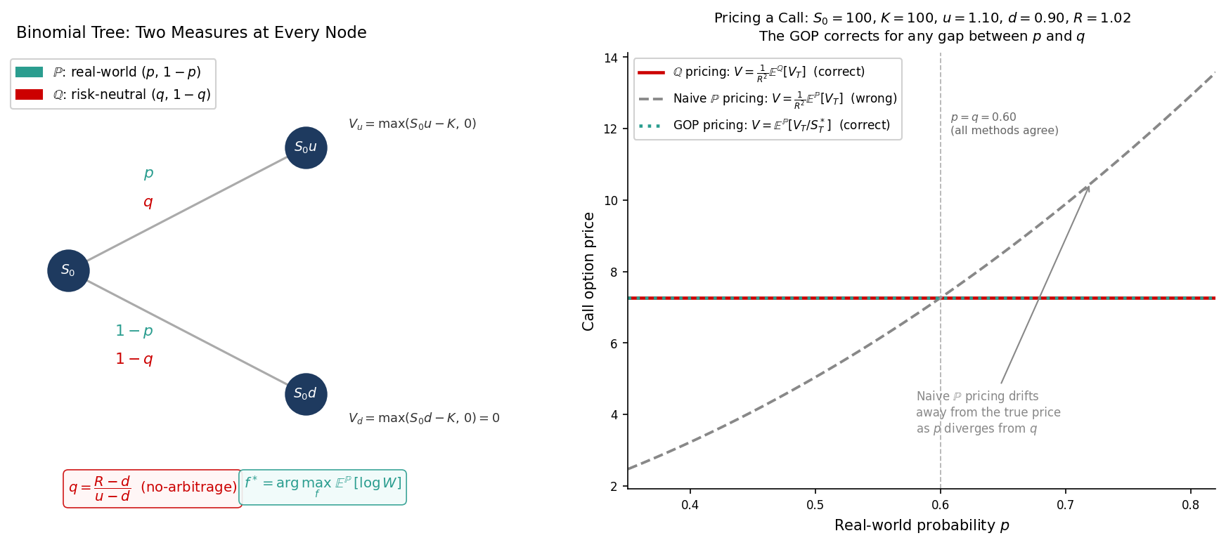
The binomial tree is the cleanest version of the option pricing argument. At each node, the stock moves up by a factor $u$ or down by a factor $d$. The real-world probability of an up move is $p$. To price a derivative, you ignore $p$ entirely and compute:
$(1)$
This $q$ is the **risk-neutral probability** — the unique probability that makes the discounted stock price a martingale. Under $\mathbb{Q}$, every asset earns the risk-free rate. The derivative price is then just a discounted expectation:
$(2)$
Tighten the time step, choose $u = e^{\sigma\sqrt{\Delta t}}$ and $d = e^{-\sigma\sqrt{\Delta t}}$, take the limit — and you get Black-Scholes. The measure $\mathbb{Q}$ is what makes the whole construction work.
But there is another way to arrive at the same price. It starts with Kelly.
Kelly Is Log-Utility
The Kelly criterion is not a rule of thumb. It is the exact solution to a specific optimisation problem: maximise the expected log of terminal wealth.
In a single-period binomial setting, a Kelly bettor allocates a fraction $f^*$ of their wealth to the risky asset. The fraction is determined by maximising:
$(3)$
The solution $f^*$ is the Kelly fraction — the optimal bet size given the true probabilities $p$ and $1-p$. This investor is not indifferent to risk. They have a specific utility function: $U(W) = \log W$. And their optimal portfolio has a name in the continuous-time literature: the **growth-optimal portfolio**, or GOP.
The Growth-Optimal Portfolio as Numeraire
The GOP has an extraordinary property. In a complete market, any tradeable asset — including a derivative — satisfies:
$(4)$
where $S^*$ is the GOP wealth process. Compare this to the standard risk-neutral formula:
$(5)$
where $B$ is the risk-free bond. Both formulas give the same price. They are two representations of the same object: one uses the risk-free bond as numeraire and prices under $\mathbb{Q}$; the other uses the GOP as numeraire and prices under the real-world measure $\mathbb{P}$.
The GOP is, in this sense, the **natural numeraire** of a log-utility investor. What the risk-free bond is to $\mathbb{Q}$, the Kelly portfolio is to $\mathbb{P}$.
The Measure Connection
The two pricing formulas are related by a change of numeraire. The Radon-Nikodym derivative connecting $\mathbb{Q}$ to $\mathbb{P}$ is:
$(6)$
This is the stochastic discount factor (SDF) of the log-utility investor, normalised to integrate to one. It tells you exactly how to go from real-world probabilities to risk-neutral ones: weight each scenario by the relative underperformance of the GOP against the bond in that scenario.
In states where the GOP did well, the $\mathbb{Q}$-weight is low. In states where the GOP lagged the bond, the $\mathbb{Q}$-weight is high. The risk-neutral measure is, literally, the Kelly investor’s marginal valuation of future states.
This is not a coincidence or a mathematical curiosity. It reflects something real: option prices embed the price of risk, and the price of risk is determined by how a log-utility investor values uncertain payoffs.
Platen’s Benchmark Approach
The real-world pricing formula (4) is not just a mathematical curiosity. It is the foundation of a complete alternative framework for derivative pricing, developed by Eckhard Platen and laid out systematically in *A Benchmark Approach to Quantitative Finance* (Platen and Heath, 2006).
The central object is the **benchmarked price**: any asset price $V_t$ expressed in units of the GOP,
$(7)$
The fundamental theorem of the benchmark approach states that for any non-negative self-financing portfolio, $\hat{V}_t$ is a **local martingale** under $\mathbb{P}$. Not under $\mathbb{Q}$ — under the real world. The GOP is the natural deflator for real-world pricing in the same way the bond is the deflator for risk-neutral pricing.
A claim is called **fair** if its benchmarked price is a true martingale (not merely a local one) under $\mathbb{P}$:
$(8)$
Substituting $\hat{V}_t = V_t / S^*_t$ and $S^*_0 = 1$ recovers equation (4) exactly. In a complete market, every contingent claim is fair, and the benchmark price coincides with the Black-Scholes price. The two frameworks are identical.
The difference emerges in incomplete markets. When $\mathbb{Q}$ is not unique, there is a family of risk-neutral measures, each producing different prices for a given payoff. The benchmark approach has no such ambiguity: the GOP is always unique, determined solely by the market structure and $\mathbb{P}$. For any contingent claim, the benchmark price is the **minimal** price consistent with no-arbitrage — the cheapest way to super-replicate the payoff.
A benchmarked price that is a strict local martingale — where $\mathbb{E}^{\mathbb{P}}[\hat{V}_T] < \hat{V}_0$ — signals a **pricing bubble** under the classical framework. Under the benchmark approach, this is not a pathology but a feature: the benchmark price is still well-defined and corresponds to the intrinsic value of the claim stripped of the bubble component. Classical risk-neutral pricing may assign a higher price to the same payoff by inadvertently including bubble value.
This has direct consequences for long-dated options, derivatives on non-replicable assets, and any setting where the market is genuinely incomplete. The risk-neutral price may overstate fair value. The benchmark price does not.
Thorp Got Here First
Ed Thorp — who built the first wearable computer to beat roulette at MIT, then systematically beat blackjack, then ran one of the most successful hedge funds in history — derived a version of the Black-Scholes formula before Black and Scholes.
His approach was not the PDE argument or the replication argument. It was a Kelly argument: if you know the true distribution of the stock, you can compute the GOP allocation, and from that, the fair price of a warrant. He arrived at the same formula from a completely different direction and chose not to publish it as a pricing result.
The fact that two distinct paths — one from no-arbitrage and one from log-utility — lead to the same formula in complete markets is not a coincidence. It is the same fact stated twice.
The Unified Picture
Three objects turn out to be the same thing: the Kelly portfolio, the growth-optimal portfolio, and Platen’s benchmark. They are different names for the unique portfolio that grows faster than any other strategy almost surely in the long run, and whose inverse — $1/S^*_t$ — serves as the natural state-price deflator under $\mathbb{P}$.
The risk-neutral measure $\mathbb{Q}$ is the tool a derivatives desk uses to price without a view on the real-world distribution. It is operationally clean: you do not need to estimate $\mu$, you only need $\sigma$ and $r$. It requires an equivalent martingale measure to exist, which requires the market to be complete or for a particular measure to be selected.
The benchmark approach is the tool that works when none of that holds. It prices under $\mathbb{P}$ using the GOP as numeraire, requires no EMM, and gives minimal fair prices. In complete markets the two approaches agree. In incomplete markets the benchmark price is the lower bound that the risk-neutral approach cannot go below without introducing arbitrage.
The binomial tree already contains all of this. The $q$ at each node is not an arbitrary choice — it is the unique probability that eliminates the need to know $p$. The thing that makes $p$ irrelevant in the risk-neutral world is exactly that a Kelly investor using $p$ would arrive at the same price via the benchmark route. The coin flip and the option pricing formula are, at their core, the same problem.
Working on a pricing model or risk system? Let’s talk.
