From Plasma to Game Theory: The Unlikely Journey of an SDE

A Self-Referential Equation

In 1938, Soviet physicist Anatoly Vlasov was studying plasma — a gas of charged particles so dense that every particle feels an electric field generated by every other. Tracking individual interactions was hopeless. Vlasov’s solution: replace the swarm with a smooth density, let each particle move in the *mean field* that density generates. The individual disappears; the collective takes over.

This idea — that the average behaviour of a crowd can stand in for the crowd itself — would resurface, in very different clothing, seventy years later.

Propagation of Chaos and the McKean-Vlasov SDE

Consider $N$ particles, each governed by a stochastic differential equation that couples it to all the others:

$$dX_t^i = b\!\left(X_t^i,\, \frac{1}{N}\sum_{j=1}^N \delta_{X_t^j}\right)dt + \sigma\!\left(X_t^i,\, \frac{1}{N}\sum_{j=1}^N \delta_{X_t^j}\right)dW_t^i$$

$(1)$

Here $\frac{1}{N}\sum_j \delta_{X_t^j}$ is the empirical measure of the system — the crowd’s fingerprint at time $t$. As $N \to \infty$, something remarkable happens. The particles *decouple*: each one becomes statistically independent, driven not by the actual crowd but by a smooth limit $\mu_t = \mathcal{L}(X_t)$, the law of a single representative particle.

This is **propagation of chaos**, a term due to Mark Kac (1956). In the limit, every particle satisfies the same **McKean-Vlasov SDE**:

$$dX_t = b(X_t,\, \mu_t)\,dt + \sigma(X_t,\, \mu_t)\,dW_t, \qquad \mu_t = \mathcal{L}(X_t)$$

$(2)$

Here $\mathcal{L}(X_t)$ denotes the **law** of $X_t$ — its probability distribution at time $t$. Concretely: if you ran the process many times independently and histogrammed the positions at time $t$, the histogram would converge to $\mathcal{L}(X_t)$. It is the same object as $\mathrm{dist}(X_t)$ or $\mathbb{P} \circ X_t^{-1}$; the $\mathcal{L}$ notation is standard in probability theory.

The equation looks circular: to solve for $X_t$ you need $\mu_t$, but $\mu_t$ is the law of $X_t$. Henry McKean showed in 1966 that this fixed-point problem is well-posed — and that it arises naturally from interacting particle systems in physics and biology. For decades it remained a beautiful result in probability theory, with roots in plasma physics and kinetic theory. Its connection to rational decision-making was not yet imagined.

Mean Field Games

In 2006, two groups working independently arrived at the same equation from a completely different direction. Jean-Michel Lasry and Pierre-Louis Lions in Paris, and Minyi Huang, Roland Malhamé, and Peter Caines in Montreal, were studying games with large populations of rational agents.

The question: what happens when $N \to \infty$ agents each optimise their own cost, and each agent’s environment is shaped by what everyone else does? In the mean field limit, no single agent is large enough to move the crowd. So each agent treats the population distribution $\mu_t$ as given and solves an individual stochastic control problem. The value function $V(t, x)$ satisfies a **Hamilton-Jacobi-Bellman equation** running backward in time:

$$-\partial_t V + H(x,\, \mu_t,\, \partial_x V) – \tfrac{1}{2}\sigma^2\,\partial_x^2 V = 0$$

$(3)$

where $H$ is the Hamiltonian encoding the agent’s cost and the interaction with $\mu_t$. The optimal control $u^*(t,x)$ is read off from the minimiser of $H$.

The second equation tracks how the population density evolves forward in time when all agents play optimally. This is the **Fokker-Planck equation**:

$$\partial_t \mu_t + \partial_x\!\left(b^*(x,\, \mu_t)\,\mu_t\right) – \tfrac{1}{2}\sigma^2\,\partial_x^2 \mu_t = 0$$

$(4)$

where $b^* = b(x, \mu_t, u^*)$ is the drift under the optimal control. Equations (3) and (4) must be solved simultaneously: (3) runs backward from a terminal condition, (4) runs forward from an initial distribution. The Nash equilibrium is the pair $(V, \mu)$ such that each equation is consistent with the other.

The Fixed Point — and Where the Paths Meet

The MFG equilibrium condition is: the distribution $\mu_t$ assumed by each agent when solving (3) must equal the distribution actually generated by optimal play in (4). This is a fixed-point problem in the space of probability measures.

At the fixed point, each individual agent’s optimal dynamics are exactly:

$$dX_t^* = b^*(X_t^*,\, \mu_t)\,dt + \sigma(X_t^*,\, \mu_t)\,dW_t, \qquad \mu_t = \mathcal{L}(X_t^*)$$

$(5)$

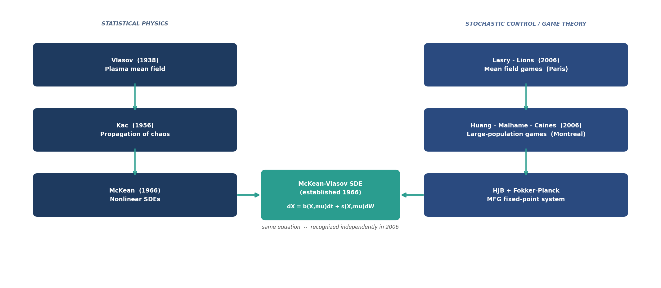
Equation (5) is the McKean-Vlasov SDE — equation (2), recovered now from the game-theoretic side. The figure below traces the two paths that converge on the same object.

**Figure 1.** Two independent traditions — statistical physics (left) and stochastic control theory (right) — converge on the McKean–Vlasov SDE from opposite directions.

Two Cultures, One Equation

The convergence is striking. McKean came from statistical mechanics, working upward from interacting particle systems toward a nonlinear, law-dependent diffusion. Lasry–Lions and Huang–Malhamé–Caines came from control theory and economics, working downward from a game with infinitely many rational players toward the same object. Neither group was following the other’s trail.

What the physics tradition contributed was the probabilistic language: propagation of chaos, weak convergence of measures, nonlinear Markov processes. What the game theory tradition contributed was the *meaning*: the McKean-Vlasov SDE is not merely the limit of a particle system, but the geometry of rational collective behaviour. Every time a large population of self-interested agents reaches a Nash equilibrium — and the game is symmetric and the population large enough — the dynamics they produce are McKean-Vlasov.

The equation Vlasov wrote to describe electrons in a star turns out to also describe speculators in a market, pedestrians in a crowd, and drivers on a motorway. Whenever there are too many agents to treat individually, and each one is, in their own small way, thinking.

Interested in this line of work? Get in touch.