The Kelly Criterion — Why the Optimal Strategy Is Never Used
A Coin With an Edge
Suppose someone offers you a coin. It lands heads 55% of the time. You can bet any fraction of your bankroll on each flip, collect if it lands heads, lose your stake if it lands tails. You can play as many times as you want.
How much do you bet?
Most people say something between 10 and 20 percent. A few say 60 percent — the probability of winning. Almost nobody says the correct answer on the first try, and almost nobody actually follows the correct answer in practice.
That answer has a name: the Kelly Criterion. It is one of the few places in all of finance and probability where the mathematically optimal strategy is known, proved, and universally ignored.
The Formula and Where It Comes From
John Kelly was a physicist at Bell Labs in 1956, working in the orbit of Claude Shannon. His paper — *A New Interpretation of Information Rate* — was ostensibly about signal transmission. What it actually contained was a complete theory of optimal betting.
The setup: you have an edge. Your probability of winning is $p$, losing is $q = 1 – p$. If you win, you collect $b$ times your stake. You bet a fixed fraction $f$ of your current bankroll each round. What fraction maximises your long-run wealth?
Kelly’s answer: maximise the expected log-wealth after $n$ bets. One round changes your wealth by a factor of $(1 + bf)$ on a win and $(1 – f)$ on a loss. The expected growth rate per round is:
$(1)$
Differentiate with respect to $f$, set to zero:
$(2)$
Solve:
$(3)$
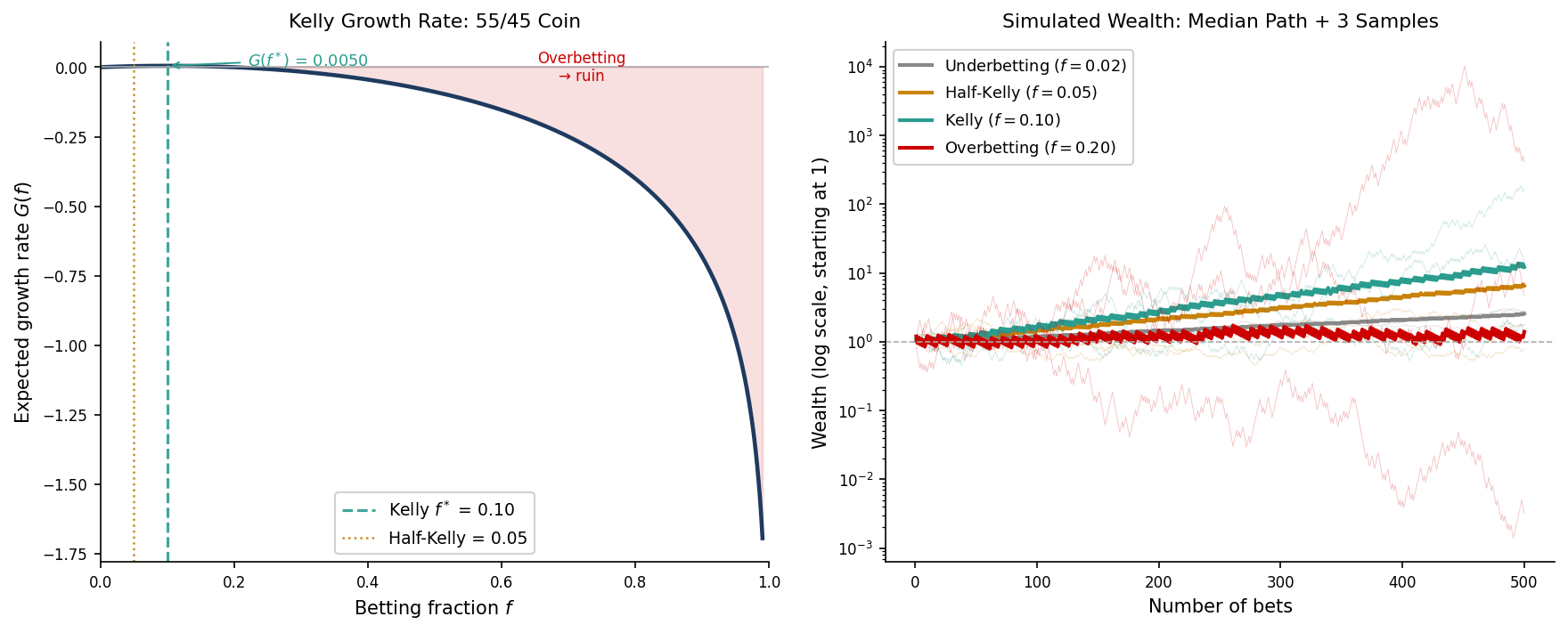
For our 55/45 coin with even odds ($b = 1$): $f^* = 0.55 – 0.45 = 0.10$. Bet 10% of your bankroll every single time.
This is not a rule of thumb. Kelly proved, via the law of large numbers, that a bettor using $f^*$ will eventually accumulate more wealth than any bettor using any other fixed fraction. Not on average — with probability one. The Kelly bettor is the guaranteed long-run winner.
The Problem With Being Right
Here is what the simulation shows that the formula does not.
On the way to winning, the Kelly bettor experiences drawdowns that would end most professional careers. A 50% drawdown — your portfolio cut in half — is not an extreme event under Kelly betting. It is routine. The mathematics guarantees the long-run outcome. It makes no promises about the journey.
The practical problem compounds when you consider that no one actually knows the true value of $p$. You think you have a 55/45 edge. Maybe you do. But if the true probability is 52/48 and you are betting as if it is 55/45, you are **overbetting Kelly**. And the growth rate curve is not symmetric: overbetting is far more damaging than underbetting by the same amount. The left side of the curve is steep. The right side drops off a cliff.
$(4)$
Overestimate your edge by 5 percentage points and you may be betting twice what you should. The asymmetry is brutal.
What Practitioners Actually Do
The answer in professional trading is **half-Kelly**: bet $f^*/2$.
At half-Kelly, the growth rate falls to roughly 75% of the Kelly optimum. But the variance of outcomes falls by a factor of four, and the typical drawdown drops from catastrophic to merely uncomfortable. For a fund manager with clients, quarterly reporting requirements, and a risk committee, this is not a concession — it is the rational choice.
The deeper point is that “optimal” depends on what you are optimising for. Kelly optimises geometric growth rate. Half-Kelly optimises the trade-off between growth and psychological and institutional survivability. These are different problems, and there is no reason to pretend they are the same one.
Ed Thorp — the mathematician who beat the casino in blackjack and then beat the market for decades — knew the Kelly formula as well as anyone alive. He used half-Kelly.
Sports Betting and Prediction Markets
The coin flip is abstract. Here is the same formula applied to something where the assumptions actually hold.
**How the odds convert**
A bookmaker offers decimal odds $D = 1.90$ on Team A. That means: bet one unit, get back 1.90 units if you win — net profit of 0.90. So $b = D – 1 = 0.90$. The market’s implied win probability is $1/D = 1/1.90 \approx 0.526$. The bookmaker is saying Team A wins just over half the time.
Your model — built on xG, defensive ratings, home advantage, injuries — says $p = 0.58$. You disagree by about 5 percentage points. That gap is your edge. Apply the formula:
$(5)$
Stake 11% of your bankroll on this match. Compare that to the 10% Kelly fraction from our 55/45 coin — the fractions are in the same range because a 5-point model edge against a sharp bookmaker is roughly the same magnitude of advantage as a 5-point edge on a fair coin. The formula is behaving consistently.
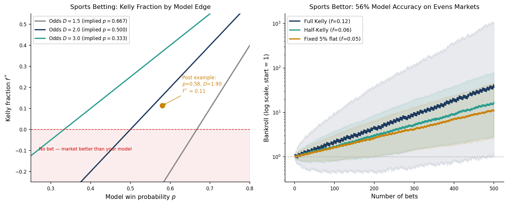
**What the left panel shows**
The figure plots Kelly fraction against your model probability for three sets of decimal odds: $D = 1.5$, $D = 2.0$, and $D = 3.0$. Each curve crosses zero at a different point — that crossing is the break-even threshold, the minimum model accuracy before a bet makes sense. For $D = 2.0$ (evens), the break-even is $p = 0.50$. For $D = 1.5$, your model needs to clear $1/1.5 = 0.667$. For $D = 3.0$, it only needs to clear $0.333$.
The red shaded zone is where $f^* < 0$: your model is below the market's implied probability, so there is no bet. The Kelly calculation disposed of it without a wager being placed.
**What the right panel shows**
500 bets at 56% model accuracy on $D = 2.0$ markets. The expected growth per bet at full Kelly is:
$(6)$
After 500 bets, the median bankroll is $e^{500 \times 0.0032} \approx 5\times$ the starting amount. Modest — which is the point. A sharp sports bettor compounds slowly and steadily, not explosively. The flat 5% stake grows too, but it falls behind over time because it does not resize as the bankroll grows. Half-Kelly sits between the two: most of the compounding benefit, far smoother paths.
**Where the figure is slightly optimistic**
The simulation uses $D = 2.0$ — true evens with no bookmaker margin. Real bookmakers do not offer this. On a genuine 50/50 match, the actual odds are typically $D = 1.88$ to $D = 1.91$, because the overround is built in. That shifts the break-even threshold from 50% to roughly 52.5%: your model needs to clear 52.5% accuracy just to have $f^* > 0$, not 50%.
This is one more reason practitioners use half-Kelly. Your estimated edge is already net of model error. It may not be fully net of the bookmaker’s cut. When in doubt, bet less.
This is where Kelly genuinely works. The outcomes are binary. The events are independent — the Champions League final has nothing to do with last week’s Serie A result. And your $p$ is a model output with a known methodology, not a retrospective statistic estimated from your own performance history. The assumptions hold. The formula applies.
The Deeper Parallel
The Kelly Criterion belongs to a small family of results in applied mathematics where a clean, closed-form optimal solution exists and is routinely overridden by rational agents for rational reasons.
The secretary problem gives you the 37% rule: ignore the first 37% of candidates, then accept the next one better than all you have seen. It is provably optimal for maximising the probability of selecting the best candidate. Almost no hiring manager follows it. Not because they are wrong — because the objective function in real hiring is not “maximise P(best candidate)”. It is something more complicated involving risk aversion, time pressure, and the cost of an empty seat.
Kelly is the same structure. The formula is correct. The objective it optimises is not always the one you actually have.
That gap — between the mathematically optimal solution and the practically tolerable one — is where most of the interesting problems in quantitative finance live.
Working on a pricing model or risk system? Let’s talk.
