Langevin Dynamics and Why They Matter in Finance

A Particle in a Noisy World

In 1908, Paul Langevin wrote down an equation to describe a small particle buffeted by the molecules of the surrounding fluid. Newton’s second law with two extra terms: a friction force opposing motion, and a random force representing molecular collisions:

The friction term $-\gamma \dot{x}$ pulls the particle back whenever it moves too fast. The noise $\xi(t)$ kicks it randomly at every instant. These two forces compete, and the particle settles into a kind of restless equilibrium — never still, never escaping.

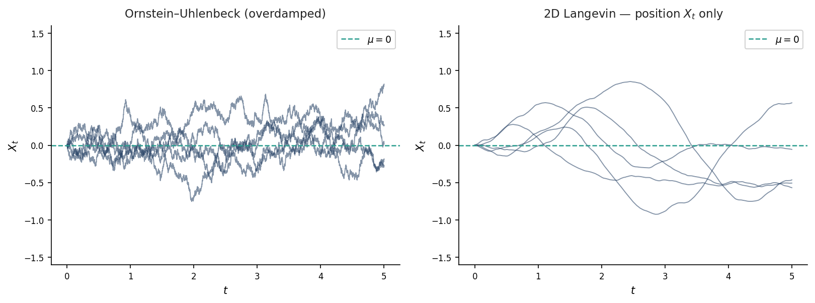
Now strip out the mass. Set $m = 0$ and let the inertia disappear entirely. What remains is the **overdamped Langevin equation** — better known in mathematics as the Ornstein-Uhlenbeck process:

The drift term $-\theta(X_t – \mu)$ pulls $X_t$ back toward $\mu$ whenever it wanders. The noise $\sigma\,dW_t$ pushes it away. This tug-of-war produces **mean reversion** — the defining feature of a process that has memory of where it came from.

Why Finance Reached for It

The Black-Scholes world models asset prices as geometric Brownian motion: they drift upward and spread without bound. That works for equities over long horizons. It does not work for **interest rates**.

Rates do not trend to infinity. When they are high, central banks and market forces push them back down. When they are low, the pressure eventually reverses. The mean-reverting OU process captures exactly this behaviour.

Vasicek (1977) was first to write it down cleanly:

The short rate $r_t$ reverts to its long-run mean $\bar{r}$ at speed $\kappa$. The stationary distribution is Gaussian with mean $\bar{r}$ and variance $\sigma^2 / 2\kappa$ — which tells you that, in the long run, rates are distributed around a central value with spread controlled by the noise-to-reversion ratio. The Vasicek model remains a foundation for yield curve modelling, despite its age, precisely because this structure is analytically tractable.

The OU process also appears in **stochastic volatility**: in the Heston model the variance $v_t$ follows a CIR process (OU reflected at zero), and in the Stein-Stein model the volatility itself follows equation (2) directly. Whenever a financial quantity should be positive on average and not drift to extremes, the OU family is the natural starting point.

The Problem with No Inertia

The overdamped OU process has one structural weakness: **it is nowhere differentiable**. Sample paths are continuous but infinitely jagged. Every increment $dX_t$ is pure noise plus an instantaneous drift correction. There is no smoothness, no momentum, no sense that where the process is going depends on where it has been heading.

For many applications this is fine. But for interest rate models, it means that the short rate can reverse direction instantaneously — no persistence in the direction of change, no inertia. Empirically, rates tend to trend for short periods before reversing. The pure OU model misses this.

Putting the Inertia Back

The full Langevin equation keeps the mass term. In SDE form, this means introducing a **velocity variable** $V_t$ alongside the position $X_t$:

Notice what is happening here. The noise $dW_t$ enters **only through the velocity equation**. Position $X_t$ is driven by velocity, not directly by a Brownian motion. $V_t$ is not an independent second source of randomness — it is the single source of randomness, filtered through the dynamics.

This is the key structural difference. The system has **one Brownian motion and two state variables**. Noise is injected once, then integrated up to produce the position path.

Why This Matters

The consequences are immediate and significant.

**Path smoothness.** Because $dX_t = V_t \, dt$, the position $X_t$ is once differentiable along every sample path. The jaggedness is in $V_t$, not in $X_t$. If $X_t$ represents an interest rate, this means the rate moves with momentum — it cannot reverse instantaneously.

**Direction persistence.** $V_t$ is itself mean-reverting (the $-\gamma V_t$ term). It retains its sign for a while before the noise flips it. This produces the short-term trending followed by long-run mean reversion that is visible in rate time series.

**Richer term structure.** In a bond pricing model built on (4)–(5), the yield curve depends on both $X_t$ and $V_t$. The current velocity of the rate contributes information about where rates are heading — not just their current level. This gives the model a term structure that can capture concave or convex shapes that single-factor OU cannot.

**Controlled noise injection.** Because noise enters only once — through $V_t$ — there is no need to calibrate two independent volatility parameters or two correlation structures. The model is parsimonious: one diffusion coefficient $\sigma$, two mean-reversion parameters $\gamma$ and $\kappa$.

From Rates to Forward Curves

The same structure extends naturally to infinite-dimensional settings. In Heath-Jarrow-Morton type models, the short rate is replaced by the entire forward rate curve $f(t, T)$. Langevin dynamics on the curve means the forward rates evolve with inertia: the velocity of each point on the curve is a state variable, noise enters through the velocity SPDE, and the curve itself moves smoothly in time.

This is the direction the Langevin-Zamrik model takes. The inertial structure is not an add-on — it is the organising principle. A physics equation written to describe a particle in a fluid turns out to be exactly the right language for describing how a yield curve should move.

Interested in this line of work? Get in touch.